Assessing UAV-based laser scanning for monitoring glacial processes and interactions at high spatial and temporal resolutions

1 Introduction

It is now widely recognised that nearly all of the world’s ∼198,000 glaciers are undergoing widespread retreat in response to continued and more intensive global climate warming (Truffer and Motyka, 2016; Farinotti et al., 2019; Zemp et al., 2019). This retreat will have a significant impact on future freshwater supplies (approximately one-third of the world’s population lives within a glacierised drainage basin), hydropower generation (fed by glacier meltwater) and global sea level rise (to which glaciers are projected to contribute substantially to over the coming century) (Huss and Hock, 2018; Farinotti et al., 2019; Shannon et al., 2019). As a result, more detailed and in-depth glacier monitoring is required to accurately quantify and project their future patterns of mass loss and retreat (Paul et al., 2015; Chernos et al., 2016; Millan et al., 2019).

However, this relationship between climate and glacier response is more complicated for those glaciers which terminate in water, because in these settings retreat is often instead controlled by an additional and highly significant mass loss mechanism termed calving (Warren and Kirkbride, 2003; Howat et al., 2007; Benn and Åström, 2018). Indeed, calving can decouple the behaviour of a glacier from climate due to feedbacks that can arise in response to changes in water depth or glacier geometry at the calving margin, meaning such glaciers have the potential to contribute disproportionately to global sea level, compared to those solely driven by climate (Howat et al., 2008; Carrivick and Tweed, 2013; Baurley et al., 2020). Such glaciers are, therefore, imperative to monitor, with the majority of our understanding of these processes stemming from the application of satellite remote sensing across a range of spatial and temporal scales (e.g., King et al., 2018; Sakakibara and Sugiyama, 2018; Dell et al., 2019). However, the relatively coarse spatial and temporal resolution of this data, and its susceptibility to cloud cover, can limit their applicability when monitoring changes over fine spatial and temporal scales (Lemos et al., 2018; Millan et al., 2019). Despite advances in recent years towards higher resolution satellites with shorter repeat intervals, it is still difficult to investigate short-term variations in calving glacier behaviour using satellite remote sensing alone (e.g., Sugiyama et al., 2015; Altena and Kääb, 2017; How et al., 2019).

The emergence of Uncrewed Aerial Vehicles (UAVs) in cryospheric research over recent years provides a sound alternative due to their ability to offer rapid assessments of glacier surface dynamics at extremely high spatial (cm) and temporal (sub-daily) resolutions (Whitehead et al., 2013; Ryan et al., 2015; Chudley et al., 2019). This method has several advantages, the primary one being that it is extremely well-suited for conducting rapid repeat surveys of the ice surface due to the ability to deploy the UAV system “on demand” (Immerzeel et al., 2014; Rossini et al., 2018). This affords glaciologists the opportunity to undertake weekly, daily, or even sub-daily surveys of the ice surface at high spatial resolutions, enhancing our ability to monitor and quantify the rapidly changing glacial landscape and how it may respond in future (e.g., Ryan et al., 2015; Benoit et al., 2019; Groos et al., 2019).

The majority of glaciological studies to date which have utilised UAVs have done so in combination with (relatively) low-cost Structure from Motion (SfM) photogrammetry, which allows for the generation of orthomosaics and Digital Elevation Models (DEMs) of the ice surface and surrounding morphology at extremely high resolutions (e.g., Bash et al., 2018; Rossini et al., 2018; Benoit et al., 2019; Yang et al., 2020). However, SfM is highly dependent on feature detectability, lighting conditions, the placement of Ground Control Points (GCPs), and the surface being surveyed, amongst other aspects, all of which can be limiting factors when surveying in glacial environments (Tonkin et al., 2014; Piermattei et al., 2015; Gindraux et al., 2017; Fugazza et al., 2018). This is especially apparent at the front of calving glaciers where shadowing, crevasse morphology, the need for various camera angles, and a lack of GCPs due to inaccessibility, can significantly reduce modelling accuracy (e.g., Ryan et al., 2015; Chudley et al., 2019; Jouvet et al., 2019).

However, recent technological advances in UAV surveying may allow several of the above limitations to be overcome. For example, the development and miniaturisation of new payloads such as compact laser scanners and motion units has provided new opportunities for the accurate investigation of cryosphere dynamics (Chudley et al., 2019; Jacobs et al., 2021). Furthermore, the development of enhanced positioning and motion units onboard these UAV systems has allowed for the implementation of a new technique, termed direct georeferencing. This enables cm-scale accuracy to be obtained without the need for the deployment of an extensive network of ground-based GCPs (e.g., Benassi et al., 2017; van der Sluijs et al., 2018), eliminating one of the key limitations of the UAV-SfM methodology in glaciology (Chudley et al., 2019; Yang et al., 2020).

To date, these new developments have shown promise in applications ranging from forestry research to river corridor monitoring (e.g., Jaakkola et al., 2010; Lin et al., 2011; Flener et al., 2013; Wallace et al., 2014; Resop et al., 2019; Tomsett and Leyland, 2021). However, their deployment within cryospheric research is still limited, with research to date focussing solely on snow depth mapping (e.g., Harder et al., 2020; Jacobs et al., 2021). Therefore, there is a need to examine the possible benefits of using UAV-based Laser Scanning (UAV-LS) in glacial research, as such systems have the potential to provide new insights into glacial processes (e.g., surface elevation changes and calving) that would be challenging to capture using traditional UAV-SfM or satellite remote sensing (Chudley et al., 2019; Jouvet et al., 2019; Śledź et al., 2021).

In this study, we assess the suitability of UAV-LS as a method for investigating short-term changes in ice surface elevation, calving front geometry and crevasse morphology by undertaking repeat surveys of the calving front of Fjallsjökull, a lake-terminating glacier in southeast Iceland. We compare our findings to those produced through current UAV-SfM techniques, which were acquired alongside the UAV-LS data, to discuss the potential benefits and limitations of both techniques and, therefore, further determine the potential of the method in glacial research. To the best of our knowledge, this is the first assessment of UAV-LS for the monitoring of dynamic glacial environments, with this study aiming to highlight the relative advantages of the method for glaciologists undertaking research in similar environments.

2 Study site

Fjallsjökull (64°01′N, 16°25′W) is an easterly-flowing piedmont outlet glacier situated on the southern slopes of the Vatnajökull Ice Cap, in southeast Iceland (Figure 1) (Evans and Twigg, 2002; Dell et al., 2019). In 2010, the glacier covered an area of ∼44.6 km², had a volume of 7.0 km³ and was ∼12.9 km long (Hannesdóttir et al., 2015). Like many glaciers in Iceland, Fjallsjökull has undergone considerable recession over the last century, retreating by ∼1.7 km between 1934 and 2019 (Hannesdóttir et al., 2015; WGMS 2020), with a particularly heightened rate of retreat observed since the early 2000s (Dell et al., 2019; Chandler et al., 2020).

FIGURE 1

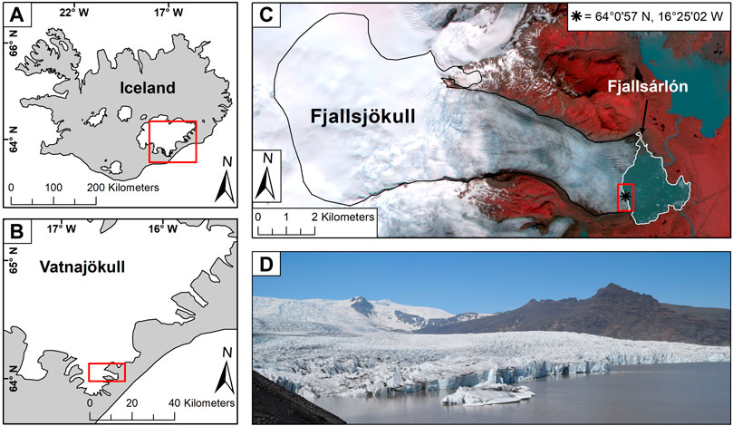
FIGURE 1. (A) Location of Fjallsjökull within Iceland, and (B) within the Vatnajökull Ice Cap. (C) Area of Fjallsjökull and Fjallsárlón as of July 2021. Red box delineates the areal coverage of the UAV surveys undertaken in this research. This is the same extent shown in Figure 2A. Background is a 4-band false-colour PlanetScope acquisition from 07/07/2021. (D) Field photograph of a portion of the calving front of Fjallsjökull, taken from the nearby lateral moraine on 15th July 2021. The calving front in the centre of the image is ∼15–20 m high, and it is over this region that our UAV surveys extend.

This ongoing retreat has revealed a substantial overdeepening, which attains a maximum depth of ∼206 m, is ∼3 km wide, and ∼4 km long (Magnússon et al., 2012; Dell et al., 2019). The emergence of this overdeepening has led to the development of the large proglacial lake Fjallsárlón (∼3.7 km² in 2018), the third largest in southeast Iceland, into which the glacier currently terminates (Guðmundsson et al., 2019; Chandler et al., 2020). Recent research by Dell et al. (2019) has shown that the deep subglacial topography and continued expansion of Fjallsárlón have become important controls on the overall ice-flow velocity and calving dynamics of the glacier, particularly over the last ∼20 years, warranting further research into this rapidly changing and highly dynamic glacier (Guðmundsson et al., 2019; Chandler et al., 2020).

3 Materials and methods

3.1 UAV design

This study used the same UAV setup as described in Tomsett and Leyland (2021), demonstrating the ability to collect topographic data in challenging fluvial environments with an accuracy of below 0.1 m. An overview of the methods and processing undertaken here are provided below, with a more detailed description of sensor integration and post-processing methods given in Tomsett and Leyland (2021).

The UAV-LS uses a Velodyne VLP-16 Puck Lite laser scanner which is compact, has a low power consumption, and is lightweight (0.59 kg), making it ideal for UAV based deployments. The sensor collects up to 300,000 points per second up to a range of 100 m with a stated accuracy of ± 0.03 m (Velodyne Lidar, 2018). Research by Glennie et al. (2016) has indicated that the sensor is stable across a range of temperatures, making it suitable for cryospheric research. A Pulse Per Second signal is provided to the laser scanner to calibrate the internal clock and avoid drift, which after 20 min of flight, if left uncorrected, could result in up to 0.37 m of positional error (when flying at 5 m s⁻¹).

Position and orientation data were obtained via an Applanix APX-15 Inertial Motion Unit (IMU), specifically designed for UAV integration. The high data collection rate of 200 Hz makes it suitable for use in direct georeferencing applications, with post-processed accuracies in the X, Y, and Z planes of 0.02–0.05 m, roll and pitch accuracies of 0.025°, and heading accuracy of 0.08° (Applanix, 2018). A single Tallysman TW3882 dual phase GNSS antenna was used to provide positional data to the APX-15 unit, mounted on top of the UAV and equipped with a mounting plate to avoid signal interference from multipath errors (e.g., Jouvet et al., 2019). A mini-PC was used to record incoming data from the laser scanner to be stored locally, as well as to collect data from the IMU. The PC was accessed via a remote connection to an external laptop, and was used to check data capture at the start and end of each flight. This was housed inside a senor box with the IMU and battery pack, which the laser scanner was then mounted to externally.

The sensor box was deployed on a DJI M600 Pro, a powerful heavy lift UAV capable of carrying loads up to 6 kg, with flight times between 15–25 min depending on the load (DJI, 2022b). The current configuration was capable of collecting 20 min of data in a single flight (including initialisation). The sensor box was attached to a mounting plate which placed the scanner in front of the main body of the UAV to avoid any shadowing and to allow it to scan across track on either side of the UAV perpendicular to the direction of travel. The mounting plate was fitted with dampeners to reduce vibration travelling from the UAV to the sensors, which can reduce accuracy (Lin et al., 2011). Offsets between sensors were measured in the lab and kept consistent between field surveys, with locating lugs ensuring consistent laser scanner placement on the sensor box. The total system weight (including a multi-spectral camera not utilised in this study) came to approximately 2.6 kg (Figure 2B).

FIGURE 2

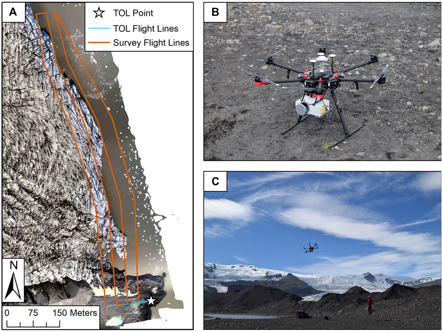
FIGURE 2. (A) Map illustrating the angled flight lines and areal coverage of the surveys flown in this study. Take-off and landing point (TOL) is given by the white star. Background is a UAV-SfM orthomosaic from 8th July 2021. (B) Our custom UAV system. The survey box, to which the laser scanner was attached, can be seen below the UAV body. This configuration was used for all surveys. (C) Example image of the initialisation procedure undertaken before each M600 survey, as recommended by Applanix.

3.2 Data collection

For this study, the survey route was pre-planned using the DJI GroundStation Pro software, using a waymarked route to fly along and over the glacier front. In order to obtain a suitable quantity of data to resolve the glacier surface and calving front, it was necessary to fly as close to the glacier as possible. However, this would increase the risk of collisions due to high surface topography, especially towards the northern extent of the study area. As a result, an initial survey was undertaken at a higher altitude to produce a model on which the original flight lines could be adjusted. These adjustments allowed for a higher resultant point density and a reduction in the impact of any orientation errors by reducing the distance from the laser scanner to the surface of interest (see Tomsett and Leyland, 2021).

Four flight lines were flown parallel to the calving front (Figure 2A), the first at the same height as the calving front [15 m Above Ground Level (AGL)] in order to capture its complex morphology from an oblique perspective, whilst the subsequent three were flown above the glacier (35–45 m AGL) to map surface features (e.g., crevasses), and to collect comparable data to a typical UAV-SfM survey (e.g., elevation changes). Although flight height should not impact the accuracy of the positioning sensors, or the range accuracy of the sensor, any boresight calibration errors and increased laser footprint size propagate errors with distance from the sensor (Tomsett and Leyland, 2021), and as such lower flight heights may be preferable. Flights were flown at 5 m s⁻¹ and covered an area of approximately 0.1 km². The survey was also designed to ensure sufficient inclusion of stable ground areas adjacent to the glacier to assess temporal model consistency, a key parameter when investigating morphological change through time. Surveys were undertaken on three separate days to identify sub-daily, daily, and weekly changes. The dates and times of these surveys can be seen in Table 1. For consistency, surveys were conducted at approximately the same time of day in both the morning and afternoon, with only one morning survey conducted on the final day.

TABLE 1

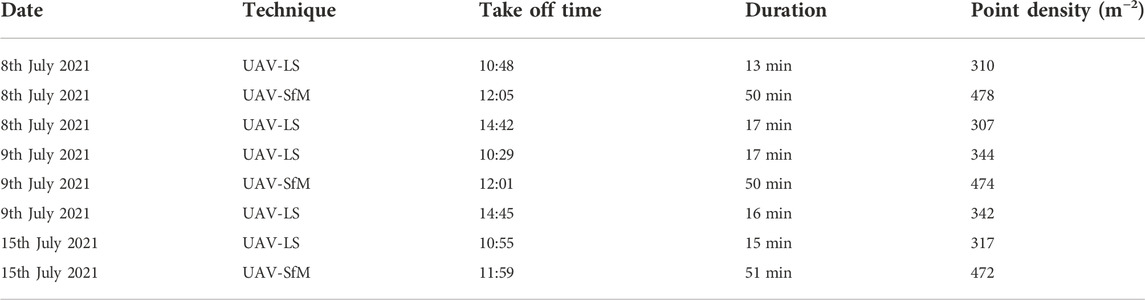
TABLE 1. Details of the UAV surveys undertaken between the 8th and 15th July 2021. For the UAV-SfM surveys, full coverage of the ∼0.9 km² study area was obtained by undertaking three individual surveys, which resulted in a total flight duration of ∼50 min.

3.3 Field workflow

In order to obtain Post-Processed Kinematic (PPK) data for the UAV, a local base station was set up for at least 4 h in the field each day. For redundancy purposes, two base stations were used in this study, a Leica GS1200 and an EMLID Reach RS2. Each base station was set up on an area of stable ground, ∼200 m from the glacier with a clear sky view and with over 10 m between the two in order to avoid any potential interference. The height of the antenna above ground level was also recorded for each base station to allow for Precise Point Positioning (PPP) post-processing using the AUSPOS online toolbox (https://gnss.ga.gov.au/auspos).

Before take-off, a 5–10 min warmup period for the IMU was required in order to improve the post-processing accuracy. Take off was then performed manually, allowing for the stability of the UAV to be checked and for the IMU to be initialised. This initialisation was undertaken by flying forwards and backwards and then side to side in an aggressive manner, aligning the IMU and calibrating the compass pre-flight (Figure 2C). The survey was then flown autonomously. After the flight path had been completed, the initialisation procedure was then repeated, before landing the UAV manually. The IMU was then left to continue logging data for another 5–10 min as done in the warm-up phase. This was repeated for each of the five survey flights across the three days.

3.4 Processing of UAV-LS data

The processing undertaken on the raw UAV-LS data consisted of three main steps: 1) Post processing of positional data, 2) Georeferencing of laser scan returns, and 3) Calibration and refinement of final point cloud data.

The creation of highly accurate PPK positional data strongly depends on the position of the user base station being precisely known. As such, the raw positional base station data was first corrected using the AUSPOS online toolbox before being used to refine the positional data of the UAV. The UAV positional processing was undertaken in the Applanix PosPac software, using forwards and backwards Kalman Filtering to produce estimates of positional accuracy throughout the duration of each flight (Kim and Bang, 2019; Scherzinger and Hutton, 2021). Once complete, the corrected data could then be exported as a time series file, which included the position, orientation and the subsequent errors of each flight, at a frequency of 200 Hz.

These data was then matched with the recorded timestamps for each individual firing of the laser scanner, so that each point could be both translated into real-world coordinates, and transformed using Euler angles to adjust the orientation of the laser scanner at the time of firing. This allows each laser scan return to be georeferenced in relation to the position of the UAV during flight. The resultant point cloud was then exported as a text file.

Finally, each point cloud was refined using the LiDAR360 programme. Flight lines were imported and segmented to remove turning points. These could then undergo a calibration procedure where each flight line had its orientation adjusted to reduce variation in the resultant point cloud surface. Once this procedure had been completed, the point cloud was cleaned within the CloudCompare Software (CloudCompare, 2020) to remove anomalous points using manual and automatic statistical outlier techniques. This procedure was then repeated for each flight.

3.5 Data quality assessment

Several studies have made use of laser scanning methods on snow and ice, both from UAV based platforms (e.g., Harder et al., 2020; Koutantou et al., 2021), as well as terrestrial and airborne measurements (e.g., Joerg et al., 2012; Bühler et al., 2016; Fischer et al., 2016; Xu et al., 2019). The setup used here has also been proven to be accurate to less than ± 0.1 m in a vegetated river corridor (Tomsett and Leyland., 2021), and as such provides confidence in the potential accuracy of the system when deployed for cryospheric applications.

In order to assess the accuracy of the setup in the present study, seven ground control points (deployed for the UAV-SfM surveys described in 3.5) were used to compare to the processed UAV-LS data. Due to the limited sample size of GCPs a comparison of the median and Normalised Median Absolute Deviation (NMAD) errors are reported for each day, as well as the median, NMAD, 68.3%, and 95% confidence intervals for all the data, as outlined by Höhle and Höhle (2009) and Bash et al. (2020), to better analyse the non-normal distribution of error.

A key aspect of sensor applicability is its precision, the ability to measure the same surface multiple times and produce a consistent result. To assess this, a repeat assessment of stable ground topography was undertaken. This uses the principle that the topography should be consistent between surveys and that any changes are indicative of the uncertainty in the system. This in turn affects the level of confidence in the datasets and the level of change that can be resolved. Indeed, as outlined above, an extensive ground control network could not be deployed due to the relative inaccessibility of the glacier surface (a common issue when undertaking UAV surveys in glacial environments, e.g., Chudley et al., 2019), meaning this stable ground assessment was essential in order to identify any errors within the point clouds.

For this assessment, an area of ice-free stable ground near the lateral margin of the glacier was selected that encompassed both shallow and steep topography and which was present in all point clouds. This region was then extracted from each individual point cloud simultaneously to avoid any potential differences in stable ground extent. Once selected, each point cloud was differenced to each of the others in a pairwise fashion within CloudCompare, using the M3C2 algorithm developed by Lague et al. (2013). This allowed the error to be assessed by comparing the median error, the NMAD, as well as visualising their distribution. These errors could then be used to identify the minimum change detection threshold between surveys, which ensured that any differences present in the point clouds represented actual change.

3.6 UAV-SfM (field surveys and processing)

Parallel to the collection of the UAV-LS data, daily UAV-SfM imagery was also obtained that covered a much larger area of the glacier, including the region encompassed by the UAV-LS surveys, using a DJI Inspire 2 equipped with a 20-megapixel Zenmuse X4S camera (DJI 2022a). Surveys were undertaken once per day immediately following the first UAV-LS survey, allowing a direct comparison of the changes across different days to be made. However, as only one flight was undertaken per day, it meant sub-daily variations could not be assessed using the UAV-SfM method. Further detail about these surveys is given in Table 2.

TABLE 2

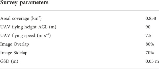
TABLE 2. Details of the flight parameters used when undertaking the UAV-SfM surveys in this study.

The UAV also had direct georeferencing capabilities, which were provided by an EMLID Reach M+ module and an external antenna, allowing the timestamp and coordinates of each image to be logged as a position file with a post-processed positional accuracy of 0.01 m (Jouvet et al., 2019; EMLID, 2022). For redundancy, however, a small network of ten ground control points (GCPs) were also deployed across stable ground near the lateral margin of the glacier ensuring a good spread in the X, Y, and Z planes. These GCPs were left at the site for the duration of the study period, with their positions recorded in the field using a Leica GS15 (to an accuracy of <0.01 m) on the 3rd July. For the final survey on the 15th July, a broken cable between the camera and the GNSS module meant no positional or timestamp information were recorded, and as such the images acquired from this day were only georeferenced using the GCPs.

To accurately post-process the GNSS data acquired by the UAV, the positional information for each survey was imported into RTKPOST_QT (https://docs.emlid.com/emlid-studio/). This was then used alongside the relevant post-processed base station file to update both the UAV track file and the positional information of each acquired image to provide camera locations accurate to <0.05 m (EMLID, 2022). Each image set was then imported into Agisoft Metashape for image alignment, with a sparse point cloud first generated. Dense point clouds were then constructed using the “aggressive” depth filtering setting, as is common in glacial research (e.g., Tonkin et al., 2014; Jouvet et al., 2019; Bash et al., 2020), before producing DEMs for each survey day. No subsequent mesh or dense cloud smoothing was performed. These were then exported at a point density of 475 points per m⁻² for the dense clouds, and a resolution of 0.05 m for the DEMs to allow for comparison with the UAV-LS data. A precision assessment was then performed over the same region of stable ground as the UAV-LS based methods, to assess the temporal consistency of the survey results using these direct georeferencing methods. This allowed direct comparisons to be made between the two methods across the same time periods of interest.

3.7 Processing of glacier-specific products

To assess the suitability of UAV-LS as a tool for glacial research, four different sets of analysis were undertaken to produce a set of glacier-specific products: 1) Changes in surface elevation, 2) Changes in calving front geometry, 3) Estimation of calving volumes and 4) Crevasse morphology and detection. Where possible, each set of analyses has been designed so that it can be compared to data obtained by current high-resolution methods over similar spatial and temporal scales, specifically UAV-SfM (See Section 3.6). In doing so, we hope to highlight some of the areas in which the use of UAV-LS may allow greater insight into key glacial processes, and glacial research more generally, than these current high-resolution methods.

3.7.1 Changes in surface elevation

To calculate the change in ice surface elevation, 2.5D DEM differencing was utilised, whereby the earlier DEM was subtracted from the latter DEM to retrieve a spatially distributed map of vertical change. For this research, the time periods investigated were sub-daily (9th am–pm), daily (8th–9th), and weekly (8th–15th), representing three distinct temporal intervals over which to test the suitability of the method. We then calculated the total volume change occurring at the ice surface for each of the three time periods investigated. This was achieved by converting each individual pixel value to a volume (multiplying by 0.0025 m² based on the DEM resolution of 0.05 m), before then summing the pixel values for each time period.

To further test the suitability of UAV-LS for quantifying changes in ice surface elevation, we compared these data to DEMs produced using UAV-SfM for the daily and weekly time period (as mentioned previously no sub-daily surveys were undertaken using the UAV-SfM method). These were first clipped to match the extent given by the respective UAV-LS-derived DEMs, before being processed as above to calculate the total volume change for both time periods.

For all periods, elevation change was only determined to be real if it was greater than the NMAD calculated during the precision assessment between the two surveys in question. This allowed a greater degree of confidence that the change being observed was real, and for the errors of each survey to be used to define the confidence intervals. These limits were reflected in the volume calculations, whereby only cells with change above this threshold were used to determine volume change.

3.7.2 Changes in calving front geometry

To assess changes in the calving front geometry, change detection was undertaken between successive calving fronts for the same time periods as investigated for the surface elevation changes analysis. This was achieved by first selecting points at the glacier terminus, before removing any points at the ice surface immediately behind the calving front, points on the water surface, and any points from the surrounding moraine, leaving only the vertical calving face of the glacier. However, because each calving front had a variable point density based on its position relative to the UAV flight lines (i.e. the front did not remain stable between surveys), a cloud-to-cloud comparison was not viable, as this may have resulted in missed points due to the absence of a point in one scan compared to another.

To overcome this, a mesh was created for each calving front using a Poisson reconstruction within CloudCompare (Kazhdan and Hoppe, 2013). This allowed for the creation of a continuous surface along each glacier front, which could then be compared to subsequent point clouds using cloud-to-mesh differencing. Before doing so, any areas that had low point densities (e.g. <six to eight points per square metre) were removed from the subsequent mesh as the confidence in the mesh reconstruction, and thus accuracy of the results, would be lower. This left some of the areas between different survey dates without comparison, however. Comparisons were again made to identify changes at the sub-daily, daily, and weekly timescales.

Alongside this, to analyse how the shape of the calving front was changing, geometric analysis of the vertical calving face was undertaken. This involved utilising functions within the CloudCompare environment to undertake surface variability analysis across the calving face as outlined in Hackel et al. (2016), providing insights into its fractured and highly variable nature. This was performed on the same segmented point clouds that had been used for the positional change analysis, with variability measured over a large 2 m focal zone. The 2 m search radius was chosen in order to identify large-scale variability in the terminal face, which may be related to calving events.

3.7.3 Estimation of individual calving events

One of the most important factors driving changes in calving front geometry is the occurrence of individual calving events. To assess the volume of subaerial ice being lost in such events, 3D volume calculations were undertaken in CloudCompare. Firstly, the results of the surface elevation and calving front geometry analysis were used to identify where large calving events had occurred. The sections of ice that were lost during such events were then separated from the main point cloud in order to reconstruct the outer surface of these blocks using a Poisson reconstruction within the CloudCompare environment (Kazhdan and Hoppe, 2013). These outer surfaces were then used to calculate the internal volume of the blocks of ice, and as such, the subaerial volume lost during that time period.

As a comparison, a 2.5D ‘raster based’ volume approach was undertaken, whereby the surface is divided into a series of pixels of a set area, and the depths of these pixels used to identify the volume per pixel, before these are accumulated to create an overall volume. This method was undertaken on both the UAV-LS and UAV-SfM point clouds for the same areas as the 3D reconstruction. No 3D approach could be undertaken on the UAV-SfM data however, because the calving front was not fully resolved by the SfM algorithms with the survey parameters used here. In each scenario, a set lake level was used that represented the lowest elevation at the front of the glacier, with an equivalent continuous surface used as the base of the 3D reconstruction for consistency between the two methods.

The main advantage of using a fully 3D method as opposed to a 2.5D method is that the 3D method can account for overhanging elements of the calving front and the surface complexity. In such scenarios, the 2.5D approach would wrongly include all areas of ‘air’ beneath the overhang as part of the glacier front, whereas the 3D approach would not. It should be noted, however, that this method is considerably more computationally intensive, and as a result, this method was only applied here to three sections of the calving front.

To assess uncertainty in the volume calculations, for the 2.5D methods a similar approach was used as for the surface elevation analysis, whereby the NMAD was used to assess the impact of uncertainty on resultant volume calculations. The approach for the 3D method was more challenging, especially given the complex nature of the surfaces. An optimal approach would run the volume calculations multiple times with errors from the precision assessment applied randomly to each point. However, this would be computationally intensive and not possible with the current non-automated workflow. Instead, a simple assumption based on volumes was used. For each block, the calculated volume was used to estimate the radius of a sphere of the same size. This was then adjusted by adding the NMAD values for weekly change, and the volume of this sphere calculated. The difference is, therefore, indicative of the uncertainty resulting from the error in the setup.

3.7.4 Crevasse morphology and detection

To compare the ability of UAV-LS and UAV-SfM data for the accurate reconstruction of crevasse morphology, transects perpendicular to ice flow were extracted from the surface of the point clouds, with a transect width of 0.5 m to enable sufficient point density. These cross sections were extracted from three locations, comprising a mix of crevasse densities, depths, and lengths, as well as from across different areas of the calving front, to encompass a variety of morphologies. All cross sections were extracted from those flights undertaken on the 9th July, using the morning flight from the UAV-LS data. The extracted scans were then visually compared and analysed, with specific focus given to the investigation of crevasse depth, to assess the differences between the two methods.

4 Results

4.1 Data quality assessment

The accuracy assessment results can be seen in Table 3. Herein, ‘F1’ refers to flight one of the day (undertaken in the morning), and ‘F2’ refers to flight two of the day (undertaken in the afternoon). Overall, the direction and magnitude of difference between the measured surface points and those from the UAV-LS are similar for flights on the 9th, and F1 on the 8th. The reduced median error for F2 on the 8th is misleading, as this shows a large deviation from the consistent difference seen in the other four flights, and has a greater NMAD of 0.115 m. Likewise, the flight on the 15th sees an increased median offset at -0.192 m indicating a change in performance, yet NMAD values are still in the same order of magnitude as the other flights, excluding F2 on the 8th. Overall, using the confidence intervals outlined by Höhle and Höhle (2009), 68.3% of the errors fall within a range of 0.118 m (0.189 m inc. F2 on the 8th) and 95% of the errors fall within a range of 0.276 m (0.399 m inc. F2 on the 8th). The low NMAD values of 0.05–0.01 m for this dataset implies that the data can be robustly used to assess real-world change, with <0.1 m offset from true values.

TABLE 3

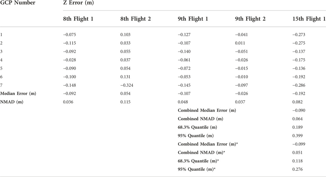
TABLE 3. Results of the accuracy assessment comparing each survey to Ground Control Points (GCPs) placed over stable ground adjacent to the glacier. These were used to assess the accuracy of each survey per day, and the overall accuracy of the surveys combined. Values marked with an * represent statistics whereby values for F2 on the 8th have been removed, due to the random error introduced throughout the survey that is discussed in 4.1.

The results of the precision assessment for the UAV-LS data (Figure 3) show values broadly in line with that expected of the system, and less than the rates of change expected at the study site (excluding F2 on the 8th, examined below), supporting the above assertion that the data is of sufficient quality to assess glaciological change over varying timescales. Comparisons between F1 on the 8th and both flights on the 9th show very good agreement, with median differences in elevation less than 0.1 m and as low as -0.004 m. The variation in these surveys is also very small, with NMADs in elevation between 0.048 m and 0.077 m.

FIGURE 3

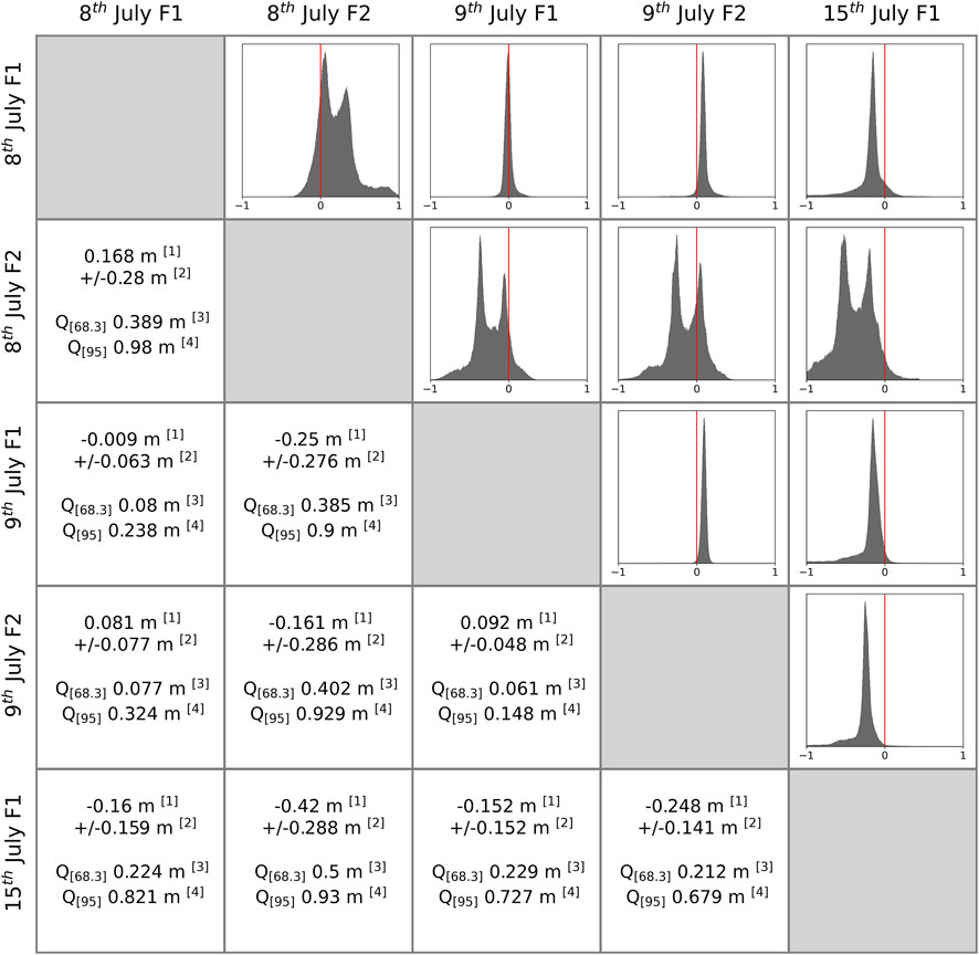
FIGURE 3. Results of the precision assessment for the UAV-LS surveys, calculated using M3C2 comparisons between each individual survey over areas of stable ground. Median^[1] and NMAD^[2] of errors are provided in the lower left of the matrix, alongside 68.3%^[3] and 95%^[4] quantiles, representing the range over which the percentage of data falls within. Histograms showing the distribution of these errors are located in the upper right of the matrix. Overall, the calculated errors are low (<0.23 m), indicating good agreement with each other, and in line with previous studies using these methods.

For the single flight undertaken on the 15th, there appears to be consistent negative offset compared to all other flights undertaken during the survey period, with a median offset of -0.152–-0.248 m when compared to F1 on the 8th and both flights on the 9th, for which there may be several potential causes. A likely prominent cause of this error is positional post-processing, where resolving accuracy in the Z direction is traditionally most complex, with errors in the range of decimetres common, especially at high latitudes where there are no-satellite zones in the sky and the majority of satellites are close to the horizon (Hugenholtz et al., 2016; Swaszek et al., 2018). This is particularly important as a reduction in the number of satellites positioned high above the horizon reduces the ability for a receiver to determine its position, especially in the Z direction (Karaim et al., 2018; Swaszek et al., 2018). Figure 4 shows the difference in satellite locations and elevations relative to the study site for the 9th and 15th July. From this, although both have a good range in satellite elevation angles, with elevations approaching 90° overhead on the 9th, the spread of satellites surrounding the study site is better for the 9th. This is seen by the lack of satellites north of the study site, with just over an 80° no-satellite zone on the 15th, compared to just under 40° on the 9th. It is also possible that errors in recording the base station height above ground level, as well as any post processing errors from the limited satellite orientation, may have propagated through to the post-processed solution. This is supported by the spread of errors being small in both the accuracy and precision assessment for the 15th (0.082 m and 0.159 m), whereas a random or non-consistent error would likely see an increase in the variation of error values (e.g. F2 on the 8th, Figure 3). As a result, the stable ground patches from the 15th were matched to those on the 9th and F1 on the 8th, using the Iterative Closest Point algorithm in CloudCompare. These offsets combined with the results of the accuracy assessment resulted in the cloud for the 15th July being vertically offset by +0.2 m, as is common in such circumstances (e.g., Lallias-Tacon et al., 2014; Williams et al., 2018; Parente et al., 2019).

FIGURE 4

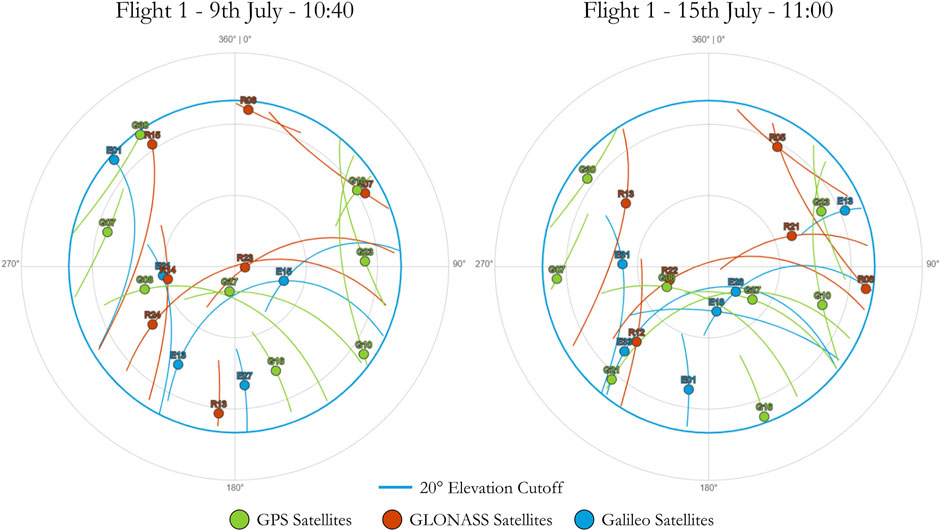
FIGURE 4. Locations of GPS, GLONASS, and Galileo satellites in the sky at the time of surveying on the 9th and 15th of July. Elevation angles of visible satellites has been set at a minimum of 20° to account for the valley sides adjacent to the glacier which would limit the viewing angles. The variation in satellite position can be seen and the effect this may have on accurately determining the position of the laser scanner, with a reduction in the number of high (closer to the crosshair) and northerly (0/360°) satellites. Data source: https://www.gnssplanning.com.

When comparing the error between F2 on the 8th and all other flight dates, there is large inconsistency in the data, with median and NMAD error values of up to 0.420 and 0.288 m obtained, respectively. Moreover, there were large increases in the quantile values when compared to the other survey dates (>0.9 m), suggesting a much greater spread of errors. Each of these comparisons show multiple peaks, suggesting that either GNSS data or calibration procedures have led to the final point cloud being incorrectly resolved. Examining the estimated errors in positional quality of the post-processed data for F2 on the 8th (Figure 5), there are large fluctuations in positional accuracy, predominantly in the Z direction, which are likely causing discrepancies in the final point cloud accuracy. These can be seen when comparing processed elevation values for F2 on the 8th and F1 on the 9th. The consistency of flight height is originally similar for both datasets, yet when there is a reduction in vertical post-processing quality, the flight height becomes more varied and stops tracking that of the heights from the 9th. It is for this reason that the second survey on the 8th was removed from all subsequent analysis.

FIGURE 5

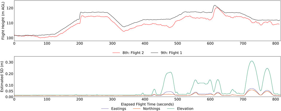
FIGURE 5. The top panel illustrates the post-processed elevation of the sensor throughout the survey for both F2 on the 8^th and F1 on the 9^th. Whilst F1 on the 9^th maintains steady elevations and smooth transitions between different prescribed flight heights, F2 on the 8^th does a much poorer job comparatively, especially towards the end of the flight. The below panel shows estimated standard deviations in positional accuracy for Eastings, Northings, and Elevation, throughout the duration of F2 on the 8th July. The position of the UAV is resolved well until midway through the flight where greater uncertainty in the post-processed position appears, with similar uncertainty in the Eastings and Northings data of around 0.05 m, but with up to 0.31 m in the Elevation data. This coincides with the increased variability of the post-processed elevation data, providing further basis to remove this survey from our analysis.

The error values presented here importantly show good agreement with those few previous studies in cryospheric research that have utilised both UAV-LS and direct georeferencing methods, as well as a similar method of accuracy assessment. For example, Harder et al. (2020) obtained values of between 0.09 and 0.10 m, and 0.13 and 0.16 m for open and vegetated snow-covered regions respectively across two sites in the Canadian Prairies. Similarly, Koutantou et al. (2021) obtained values of between 0.10 and 0.19 m for their investigation of snow depth mapping in both flat and steep forested regions of the Swiss Alps. Outside of cryospheric research, such setups have reported accuracies of between 0.04 and 0.1 m (e.g., Lin et al., 2019; Dreier et al., 2021; Tomsett and Leyland, 2021), showing our data to be in line with current methods.

In comparison, the results of the stable ground accuracy assessment undertaken on the UAV-SfM data display similar levels of consistency between surveys (Figure 6). Between the 8th and 9th, the median error between points was -0.096 m (∼3 GSD), with an NMAD of ± 0.13 m, showing that the difference between the surfaces was small across stable ground. However, for the flight on the 15th, where direct georeferencing was not possible and only GCPs could be used for georeferencing purposes, both the median error and variation in error increases, up to 0.235 (7.5 GSD) m and an NMAD of over 0.25 m. Although the 68.3% quantiles for the 15th are only 0.15–0.2 m higher, for the 95% quantile they are an order of magnitude higher. The distribution of these errors consistently shows significant variation around the median, with up to and over 1 m in difference between surveys, whereas between the 8th and 9th, these errors were more closely clustered around the median error. As a result, comparisons made to the 15th July should be interpreted with a higher degree of uncertainty than those utilising surveys from the 8th and 9th.

FIGURE 6

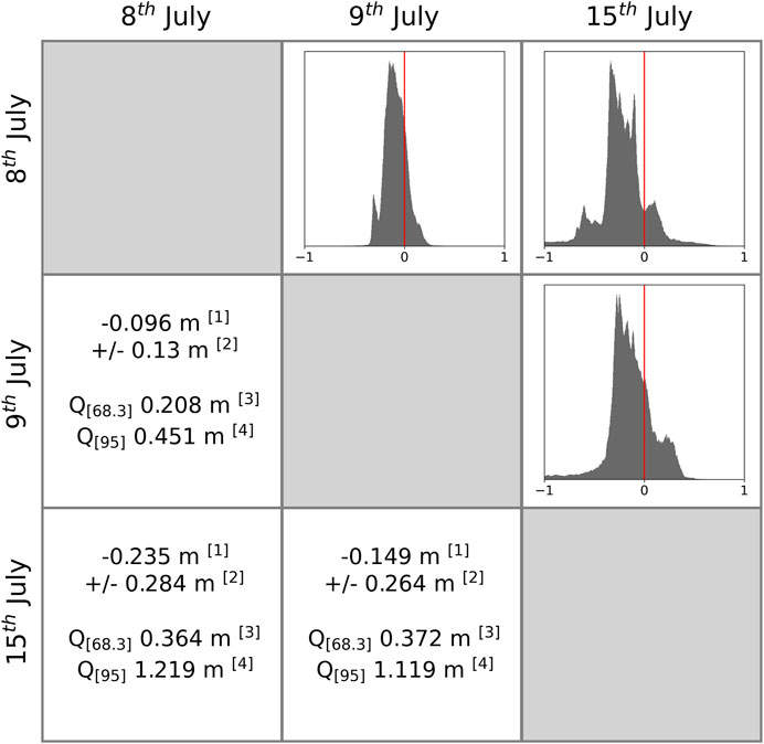
FIGURE 6. Results of the precision assessment for the UAV-SfM data, undertaken over the same areas of stable ground used for the UAV-LS data. Comparisons between data on the 8th and 9th show good agreement, with a low mean error, however, comparisons with the 15th July show a higher mean error and a greater variation in error values also, indicating a worse model performance. As previously, the Median^[1], NMAD^[2], 68.3%^[3] quantile, and 95%^[4] quantile of errors are shown.

Importantly, the errors from the 8th and 9th show good agreement with those previous studies within glaciology that have undertaken their own UAV-SfM surveys at similar flying heights to those undertaken here, while those from the 15th also show fairly good agreement. Across these studies, the range of reported errors was between 1.5 and ∼6 times the GSD, with the flying heights of each respective survey ranging between 50 m and 135 m (Wigmore and Mark, 2017; Bash et al., 2018, 2020; Rossini et al., 2018; Groos et al., 2019; Xue et al., 2021).

Overall, the results of the accuracy assessment indicate that the errors found for all surveys across both methods are smaller than the change expected over each period of interest, and are thus well within the realm of acceptability. For example, UAV-SfM surveys undertaken in July and September 2019, and July 2021 by Baurley (2022), indicate that this region of Fjallsjökull is undergoing ∼0.38 m d⁻¹ of surface thinning, and ∼0.5 m d⁻¹ of frontal position change. This means that the point clouds and DEMs generated from these surveys can be reliably used to undertake further analysis of several different glaciological processes.

4.2 Changes in surface elevation

Changes in surface elevation have occurred over each period of interest in both the UAV-LS and UAV-SfM differenced DEMs (Figure 7), although the pattern and magnitude of surface change varies between the results of both methods. Overall, the changes observed using the UAV-LS DEMs are more consistent, whilst those observed using the UAV-SfM DEMs are considerably more variable, with large extremes between the two time periods investigated.

FIGURE 7

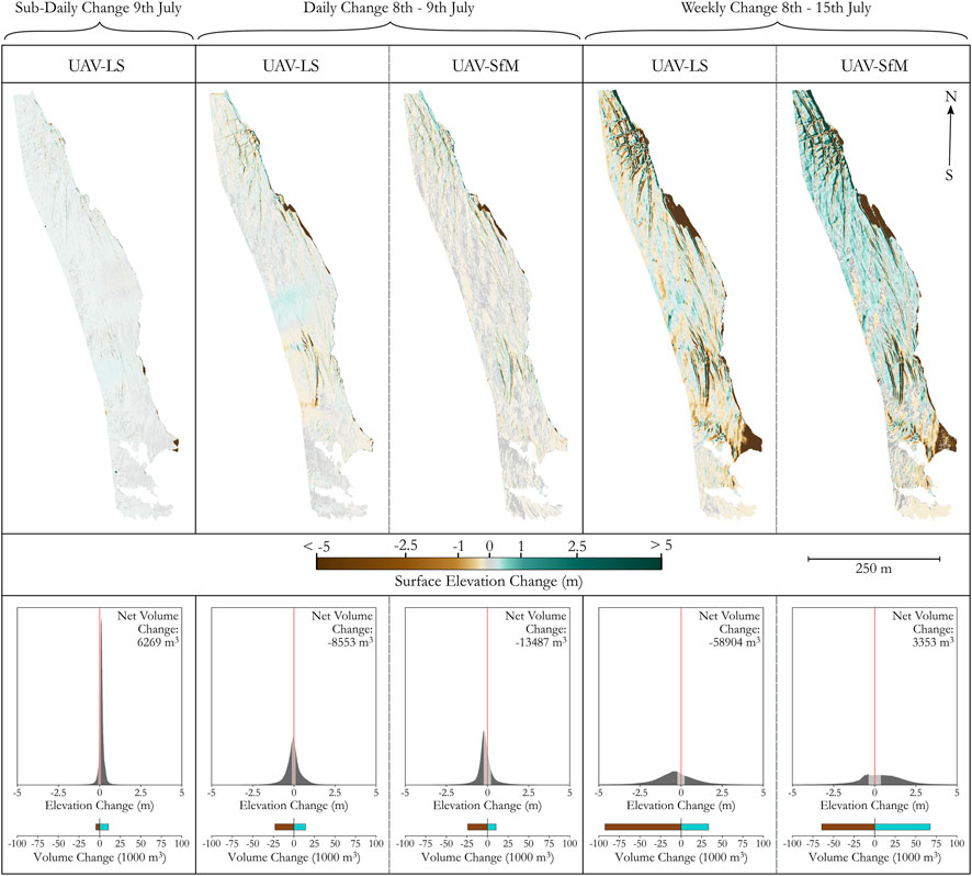
FIGURE 7. Results of the surface elevation change analysis, carried out using DEM differencing for different time periods for both the UAV-LS and UAV-SfM-derived DEMs. The upper panels show the spatial variation in elevation differences across the glacier surface. Areas in grey represent change below the NMAD analysis for each comparison outlined in Figure 4 and Figure 6. These grey areas are highlighted within the histogram panels, showing the number of pixels where change is less than the precision of the sensor. Total volume change for each time period is also shown next to the distribution of change, as well as the total loss and gain respectively for each method over each time period. This net volume change excludes any change below the limit of detection between each survey pair, i.e. excluding change within grey areas.

4.2.1 Sub-daily change

Sub-daily changes observed by repeat surveys on the 9th are muted, with very little variation in surface elevation occurring within this period. There is evidence of slightly positive change across large sections of the study region (0.01–0.2 m), although the majority of this is less than the limit of detection based on these survey dates. However, towards the southern edge of the study region, small areas of elevation loss can be observed, which likely represent calving events. Interestingly, the overall volume loss resulting from these events is less than the total surface gain observed over the study region, with the ice surface thickening by ∼6,269 m³ during this time.

4.2.2 Daily change

Towards the southern extent of the study region, both the UAV-LS and UAV-SfM data both exhibit relatively little change in surface elevation, with some small areas of ice loss observed in the UAV-LS data at the glacier front. However, to the north of this location, an area characterised by relatively high negative surface changes is present in the UAV-LS data, where over 1 m of elevation loss is observed in places, while a similar pattern is also highlighted in the UAV-SfM data for the same period. In contrast, towards the centre of the study region the UAV-LS data is characterised by an area of increasing surface elevation, with between 0.4 and 1.2 m of positive change recorded, yet there is no such pattern observed in the UAV-SfM data. Further north of this, both methods capture the large calving event that occurred at the terminus in this region, but again only the UAV-LS highlights the greater variation in surface elevation observed towards the top extent of the study region during this time. Whilst both methods accurately identify the variable nature of this heavily crevassed zone, and show visually similar patterns, the resultant loss in net volume is almost double for the UAV-SfM method at ∼13,500 m³, compared to ∼8,500 m³ for the UAV-LS data. Both the histograms and net loss and gain for this period imply that both methods have identified similar volumes of ice loss, however, the difference in net volume loss is likely due to the SfM method not detecting any regions of surface gain that occurred during this period.

4.2.3 Weekly change

Both the UAV-LS and UAV-SfM datasets show considerable differences in their patterns of surface elevation between the 8th and 15th. Both methods accurately detect the two major calving events that occurred over the study region during this time, whilst they are also able to capture the complex changes occurring in the heavily crevassed zones towards the middle and upper areas of the study region. However, whilst the UAV-LS data highlights an overall pattern of negative surface change across the study region during this time, the UAV-SfM data illustrates the opposite. In the UAV-LS data, such a pattern has likely resulted from a combination of surface ablation (e.g., Purdie et al., 2008; Trüssel et al., 2013) and dynamic feedbacks that can result from calving processes (e.g., Tsutaki et al., 2013; Shapero et al., 2016) which cause the ice surface to thin, whilst some small variations may also arise from the advection of ice down-glacier (e.g., crevasses) through time (Wigmore and Mark, 2017).

In comparison, the pattern observed in the UAV-SfM data can likely be attributed to the lack of GNSS input for direct georeferencing during the survey on the 15th. This can be seen in the histogram and net gain and loss bar chart in Figure 7, whereby there appears to be a positive shift in the results, with a greater concentration of positive change towards the northern extent of the glacier terminus. As the GCPs were placed on stable ground near the southern grounded margin, it is likely that for this survey the transformations from model to real world coordinates resulted in a tilting or doming of the model with distance away from the GCPs, increasing model uncertainty with distance across glacier (e.g., James and Robson, 2012; Micheletti et al., 2015), reducing confidence in these observations. This has resulted in an overall volume gain over the study region of ∼3,500 m³, whereas for the UAV-LS data an overall decrease in volume of ∼60,000 m³ is observed.

Overall, the accuracy of the net changes in volume cannot be corroborated, as no direct measurements could be taken of the glacier surface. However, these results importantly highlight that for the same region, surveyed on the same days, with two different methods, order of magnitude differences in volume change can be identified despite similar visual patterns of change being observed.

4.3 Changes in calving front geometry

The change in both the position and geometry of the calving front over sub-daily, daily, and weekly time periods is shown in Figure 8. It should be noted that due to the UAV-SfM surveys not adequately capturing the front of the glacier (because all imagery was acquired from a nadir perspective), this analysis is only performed on the UAV-LS data.

FIGURE 8

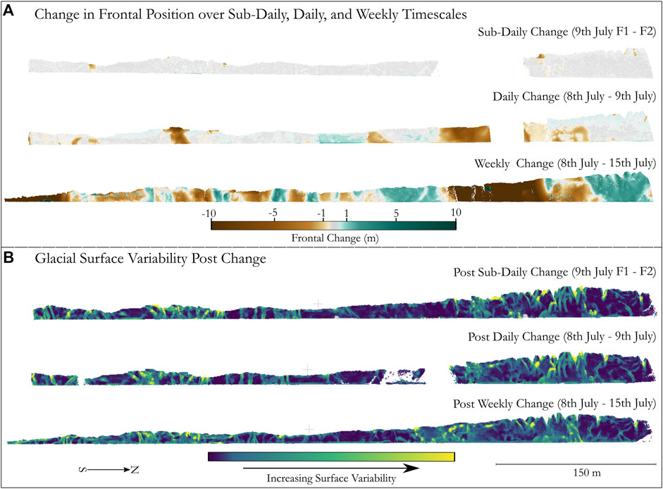
FIGURE 8. (A) Changes in the position of the calving front for the three time periods of interest. The brown, grey, and blue regions represent calving events, change less than the level of detection from the setup for those two surveys, and regions of terminus advance, respectively. Gaps in the data are due to an insufficient density of data points to accurately interpolate the calving front. (B) Changes in calving front geometry across the three time periods of interest. Geometries are representative of the surface variation at the end of each time period shown. Values in yellow indicate a higher degree of surface variation, and as such a less planar surface, with darker blues indicating a smoother, flatter surface. Areas where the point density was too low to obtain an accurate representation of the surface have been removed. Surface variability is given without scale here, and is based on a comparison of the eigenvalues obtained from a PCA of the geometry of a cloud surrounding an individual point (see Hackel et al., 2016).

The sub-daily variations illustrate that the position of the calving front changed very little during this period, similar to the results of the surface elevation change analysis. However, within this overall pattern several small calving events can also be seen to have occurred during this time, as indicated by the patches of brown along the top of the calving front.

In comparison, greater variability in the position of the calving front is observed across the daily time period. For example, several calving events occurred during this time, causing up to 5 m of terminus retreat in some locations, with these events corresponding closely to those areas of mass loss observed at the terminus in the surface elevation change analysis. Towards the centre of the calving front a region of localised terminus advance can also be observed, however, much of the glacier front has remained stable over this period or has undergone change less than the minimum level of detection offered by the UAV-LS method.

Finally, over the weekly period of monitoring, several particularly large calving events have occurred, with these again corresponding closely to the results of the surface elevation analysis. These events are between 50–100 m in length and result in localised terminus recession of over 10 m in places. Alongside these large events, several smaller regions of terminus retreat, as well as terminus advance, can also be observed across the entire length of the calving front. Such a complex pattern of terminus advance and retreat is a result of two processes: 1) glacier calving, which causes the terminus to recede, and 2) the ice velocity, which drives the calving front forward (Benn et al., 2007). Indeed, using the distance values produced in this analysis, as well as the M3C2 software, we have been able to calculate average velocities of ∼0.6 m d⁻¹ across the calving front, and although a full analysis is beyond the scope of this paper, this finding further highlights the potential applications of the method for future research.

When assessing how the geometry of the calving front has changed through time, it is noticeable that there is considerable variability across the entire length of the terminus (Figure 8B). Across each period, much of the terminus is characterised by high surface variability, particularly towards the south and north of the study region (left and right side of the figure respectively), reflecting the fractured and uneven nature of the calving face. Interestingly, these regions coincide with the location of many of the calving events shown in Figure 8A, suggesting that higher surface variability both makes these regions more susceptible to fracture propagation and thus calving (Mallalieu et al., 2020), as well as calving events leaving a fractured calving face. In contrast, those regions exhibiting lower surface variability, and thus reflecting a smoother calving face (e.g., towards the middle and north of the study region), seem to correspond well to those regions of the terminus that underwent terminus advance in this period, likely reflecting their comparable insusceptibility.

4.4 Estimation of individual calving events

The results of the calving volume estimation analysis indicate that when compared to 3D measurements of volume, the 2.5D estimations seem to overestimate the volume of ice that has been lost overall (Table 4). Only Block 1 recorded a smaller volume of ice being lost using 2.5D rather than 3D methods, with a 4.1% reduction in estimated volume loss. Furthermore, when using UAV-SfM data to estimate calving volumes, it has resulted in higher percentage differences in volume loss than for UAV-LS, with up to an 18.2% difference in ice volume estimations.

TABLE 4

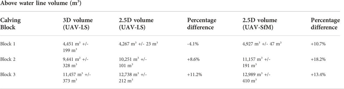
TABLE 4. Descriptive statistics showing the volume loss relating to the three calving blocks shown in Figure 9. For each event, the volumes calculated using both 3D and 2.5D techniques on the UAV-LS and UAV-SfM datasets are presented. Percentage difference column refers to the difference between the 2.5D volumes for both UAV-LS and UAV-SfM methods to the UAV-LS 3D volume. The ± values are based off the NMAD values for the weekly change detection in Figure 3 and Figure 6.

It is important to note that there are limitations when comparing UAV-LS 3D and UAV-SfM 2D data, as variability in both the method and the acquisition of data make it challenging to determine the precise nature of these differences. When comparing the performance of the two UAV-LS methods, Block 1 has a smoother and more uniform vertical calving face than the highly variable and uneven face characterised by Blocks 2 and 3, as illustrated in Figure 9. This supports the idea that a 3D volume method may be more appropriate as it can account for overhanging ice, as well as more complex surface features, which when accumulated over large areas can lead to significant differences in volume estimation.

FIGURE 9

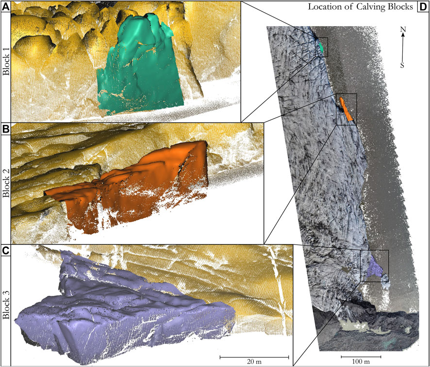
FIGURE 9. (A) Block 1, a tall block of ice located in the deeply crevassed northern region of the study site, (B) Block 2, a thinner section of ice at the front of a series of large parallel crevasses, (C) Block 3, a shorter but larger section of ice extending out at the southern margin of the glacier, and (D) An overview of the location of calving blocks 1, 2, and 3, used in the comparison of estimating individual calving events.

In contrast, when comparing the 2.5D data from both methods, it is notable that using different data sources to study the same region undergoing the same morphological change may lead to results that are not in close agreement. In the absence of reliable ground truth data with which to determine the size of these events, it is difficult to state with certainty which of the two approaches is the most suitable for the accurate quantification of calving volumes. However, the ability of the UAV-LS method to reconstruct the 3D geometry of the individual calved blocks indicates that this is likely to be the most accurate approach for the estimation of calving volume. This analysis has also highlighted the importance of understanding methodological implications, and the impact this can have on results.

The uncertainty related to the volume calculations is two orders of magnitude smaller than the estimated losses in nearly all examples. The exception to this is Block 1 for the 3D method, where the confidence intervals are one order of magnitude less but still equates to under ± 5% of the original estimated volume. The effect that error has on smaller 3D volume calculations is not linear, and therefore, the same absolute value of uncertainty will have a bigger impact on smaller blocks. This effect is not present in the 2.5D approach. The higher uncertainty in the volume calculations will also be partly due to the simplistic approach used here. Regardless, the lower uncertainty values relative to the block sizes provides confidence in using these methods in future.

4.5 Crevasse morphology and detection

The cross sections extracted from both the UAV-LS and UAV-SfM point clouds can be seen in Figure 10, with the three transects shown relative to their location on the glacier surface. The most notable difference between the two methods is their ability to reconstruct the calving front, with variable point densities resolved between the two methods across the different transects. Indeed, across all three transects, the calving front has only been partially reconstructed in the UAV-SfM data, whereas it has been reconstructed entirely in the UAV-LS data. This is exemplified in Transect 1, whereby the SfM struggles to recreate the overhang that can be observed in the UAV-LS data, resulting in a gap in the vertical profile, an issue that is present to a similar extent in Transects 2 and 3. We note that in this study the UAV-SfM surveys may have better reconstructed the calving front had they been captured from both a nadir and non-nadir perspective. However, this was not possible due to the UAV and camera model setup used, alongside limited battery life, whilst it is also often more challenging to acquire both image types in one survey due to the need for high overlap and pixel spacing between different camera angles at these scales. This is discussed in more detail in Section 5.1.

FIGURE 10

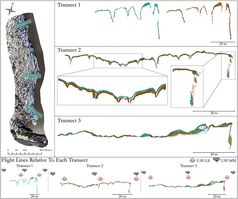
FIGURE 10. Transects across the glacier extracted from UAV-LS (brown) and UAV-SfM (blue) point clouds for the 9th July. Each transect compromises a different region of the glacier characterised by different crevasse morphologies. The location of each transect on the glacier surface can be seen in the left panel. The lower panel shows the flight paths above each of the transects (not to scale) to illustrate the position of both sensors mid-survey relative to the crevasse network, indicating good consistency between sensor locations across each transect.

In comparison, the surface of the glacier is reconstructed well overall, providing a similar profile for both the UAV-LS and UAV-SfM methods, with a variety of different crevasse morphologies detected. However, the ability to detect individual crevasse depths is not consistent between the methods. For large crevasses, both the UAV-LS and UAV-SfM pick out the location of and track the upper sections of the crevasse walls well, with the deepest crevasses being reconstructed to a greater extent in general by the UAV-LS, such as in Transect 1. However, limited surface reflections from the laser scanner due to different incidence angles of the UAV-LS surveys has meant some of the deepest crevasses and their walls have not been completely resolved in comparison to UAV-SfM, as can also be seen in Transect 1.

In comparison, when investigating smaller crevasses and surface features, there is a greater difference in the performance of the two methods. The UAV-LS appears to be better equipped to detect these small variations in surface morphology, which is illustrated by the inset of Transect 2. Indeed, the UAV-LS reconstructs several small crevasses across this transect, yet these same features have been smoothed over by the UAV-SfM methods, removing them from the analysis. This is most likely caused by the filtering and smoothing algorithms within the SfM processing workflow (Westoby et al., 2012; Smith and Vericat, 2015; James et al., 2017), but when aggregated to net volume change over large areas or for when detecting surface crevasses, may reduce the accuracy of the end results.

It is also worth noting that differences in crevasse detection will be dependent on the viewing angle of the platform (i.e., whether the crevasse is underneath the UAV or at the edge of the field of view). Figure 10 illustrates the approximate flight lines of both UAV methods relative to the ice surface, and in the majority of cases the overlap between UAV-LS and UAV-SfM flight lines is broadly similar. As a result, it can be assumed that any differences in flight lines are not a major contributor to the observed differences in reconstruction between both methods.

5 Discussion

The overall aim of this study was to assess the suitability of UAV-LS for glacial research by investigating a variety of glacial processes across differing temporal resolutions. In this section, we first compare the performance of the new UAV-LS based method to the more established method of UAV-SfM, before assessing some of the current limitations of UAV-LS for glacial applications, after which we finally suggest some avenues for future work that may benefit from the use of UAV-LS.

5.1 Comparison of UAV-LS and UAV-SfM methods for monitoring glacier change

A primary aim of this study was to highlight the potential of UAV-LS for glacial research by comparing it to the well-established and frequently used method of UAV-SfM. This allows for an understanding of which methods may be most suitable, depending on the needs of the user, and the processes that they are investigating to be developed. Herein, a discussion of the different outputs from Section 4 are presented, commenting on the suitability of both UAV-LS and UAV-SfM methods in each case.

At the surface of a glacier, an understanding of crevasse morphology can be used to inform about several different glacial processes, such as its velocity and overall structural evolution, as well as for the prediction of calving events and the stability of calving glaciers more generally, among many others (e.g., Benn et al., 2007; Tsutaki et al., 2013; Jennings et al., 2014; Benn and Åström, 2018). Yet obtaining detailed data on crevasse structure is difficult. When utilising UAV-SfM, although it is possible to reconstruct crevasses when there is large separation between opposing walls and adequate lighting (Figure 10, Transect 1), in areas where the spacing is smaller and lighting conditions are less favourable the crevasses are less well reconstructed, tending to be smoothed over or missed entirely (Figure 10, Transect 2) (Bemis et al., 2014; Ryan et al., 2015; Mallalieu et al., 2017). This is also exacerbated by the flight lines, whereby although high overlap during UAV-SfM is advised and followed in this study, this is not always possible, resulting in crevasse walls not having enough detectable features to be reconstructed (Westoby et al., 2012; Mallalieu et al., 2017; Chudley et al., 2019).

In contrast, the active rather than passive sensing of UAV-LS means that broadly consistent point coverage is acquired regardless of environmental conditions, whilst multiple viewpoints of one feature are also not required for accurate reconstruction (Li et al., 2019; Harder et al., 2020). As such, smaller variations in morphology, such as the crevasses missed by the SfM method are better reconstructed, whilst the method is also in general better able to reconstruct the morphology of the deepest crevasses. This may help to not only improve our knowledge of how such features form and evolve on the ice surface over time, but will also provide further insight into the key control such features can have on other, important glaciological processes, such as calving (Nick et al., 2010; Benn and Åström, 2018). However, where the angle of incidence is high (i.e., not perpendicular to the surface), as would be expected in deep crevasses, the ability of the scanner to detect laser returns is reduced, noticeable in both transects 1 and 2 of Figure 10. Regardless, for the transects presented in this study the use of UAV-LS still demonstrates an improvement in our ability to detect and reconstruct crevasse morphology over current UAV-SfM methods, especially given the similar flight lines. This agrees with those previous studies within glaciology that have also illustrated the difficulties in reconstructing crevasse depth when using UAV-SfM (e.g., Ryan et al., 2015; Chudley et al., 2019).

Alongside the ability to reconstruct the ice surface and related ice surface features, an equally important region to survey and investigate is the calving front itself. Accurately reconstructing these regions has remained a consistent challenge within glaciology, with the nadir viewing angles of both satellite imagery, as well as many UAV-SfM surveys, making them difficult to reconstruct due to their variable and evolving nature, large overhangs, and inconsistent geometry (Mallalieu et al., 2017; Chudley et al., 2019). To date, most studies within glaciology that have utilised UAV-SfM have typically done so using a nadir or slightly off-nadir camera angle to ensure optimal image coverage, overlap, and consistent pixel sizing (e.g., Ryan et al., 2015; Rossini et al., 2018; Yang et al., 2020). However, because calving fronts are inherently complex, with several metres of height variation across relatively small sections of imagery, reconstructing these regions using UAV-SfM can pose several challenges. This is exemplified in Figure 10, which illustrates an incomplete reconstruction of the glacier front from UAV-SfM, especially in those regions where the geometry is most complex. Furthermore, although this issue could be resolved to some extent by using dedicated non-nadir flightlines, due to the complex nature of the calving front several passes at different elevations would be required to ensure complete reconstruction.

As was the case with the reconstruction of surface crevasses, this is due to differences in the passive and active sensing nature of both methods, whereby the UAV-LS can detect features on a single pass due to the lower flying heights and the 360° data capture viewing angle of the laser scanner (Resop et al., 2019; Harder et al., 2020). This improves point densities and allows for a near complete reconstruction of the calving front. The main advantage of this is that it presents a complete view of spatially varying frontal change across different temporal scales. For example, instead of measuring differences between successive frontal positions, it is possible to identify how frontal position has changed along, and at various heights of, the glacier front, providing a 2D rather than 1D perspective of change. As a result, analysis of surface complexity (Figure 8B) and subsequent frontal change (Figure 8A) can be investigated. It is important to note that our UAV-SfM surveys were designed to be nadir-facing, and therefore, are not wholly representative of the potential ability of the method to adequately capture the calving front. However, although camera systems can be mounted on gimbals which would allow non-nadir imagery of the glacier front to be obtained, subsequently matching this imagery with nadir imagery captured from above the glacier would require sufficient overlap and matching of pixel resolutions (Westoby et al., 2012; Micheletti et al., 2015), requiring extremely detailed flight planning and potentially limiting areal coverage of the survey. This may perhaps explain why no study to date has attempted to capture the calving front using a combination of both nadir and non-nadir imagery, but we believe this should be a priority for future studies. Consequently, based off our data, the additional difficulties faced when deploying UAV-LS in this scenario are outweighed by the ability to obtain increased calving front point densities, especially when compared to the potential difficulty in acquiring suitable imagery from UAV-SfM for calving front reconstruction.

A key benefit of accurately reconstructing the calving front is the ability to calculate the volume of sub-aerial ice lost during individual calving events. Typically, to estimate calving loss a 2.5D approach would be undertaken, whereby a calved block is discretised into a 2D grid before calculating the volume of each grid square compared to a base level (in this case the lake surface) and summed. This presents an efficient method for calculating volumes, and one which has been used consistently across geomorphological applications (e.g., Wheaton et al., 2010; Williams, 2012; Whitehead et al., 2013; Jouvet et al., 2019). However, considering the complex nature of the calving front, it can be assumed that the 2.5D approach is likely to overestimate the actual volume of sub-aerial ice being lost. The differences in volume between the three methods were, therefore, as expected, with the lowest volumes for each block found for the 3D approach overall, which is better able to contour to the shape of the surface and does not include empty air beneath an overhang. In contrast, the largest estimations of ice loss were found for both 2.5D approaches using the UAV-LS and UAV-SfM methods, however, the estimated volumes were consistently higher for the latter.

This is likely due to the ability of UAV-LS to detect greater surface variation and to better identify the edge of the calving front, whereas UAV-SfM will tend to smooth over some of these variations (e.g., Smith and Vericat, 2015; James et al., 2017; Mallalieu et al., 2017). Interestingly, the reduced surface variability of Block 1 (Figure 9) suggests that for those blocks where there is limited structural complexity, a 2.5D approach is adequate for estimating sub-aerial volumes, having the smallest difference in volume estimations between the three approaches. However, what is notable is that not only is the method used to determine volume loss important, but also the original data source used, with large differences in calving volume between 2.5D UAV-LS and UAV-SfM methods observed, which has implications for future investigations of the total ice loss occurring at front of calving glaciers. It is important to note that all these approaches only consider the sub-aerial portion of ice, and the increasing complexity in fitting 3D surfaces to point clouds is computationally intensive and requires manual inspection, both of which are issues not faced by the 2.5D approach.

All three of the analyses discussed above tie into the variable results from the DEM differencing analysis, illustrated in Figure 7. What can be observed from these data is that both methods adequately capture the large changes in ice loss that occur at the calving front in both the daily and weekly comparisons, with similar locations and magnitudes recorded. This is as expected as the level of detection for both methods is lower than the magnitude of change observed across each period (Baurley (2022) observed up to ∼0.38 m d⁻¹ of surface thinning in this region in July 2021). Yet when analysing the daily variations, the changes in elevation observed across the crevassed areas are far greater for the UAV-LS than the UAV-SfM, although without extensive ground truthing it cannot be stated with certainty which method has produced the most accurate results. However, based on the crevasse detection analysis, the UAV-LS data has consistently been shown to detect more of the smaller crevasse features, as well as improving the depth to which the deepest crevasses can be reconstructed. As such, the enhanced ability to reconstruct the true elevation of the ice surface suggests that the change in elevation data acquired from the UAV-LS is a better representation of reality. This has implications for assessing net volume change, whereby smoothed SfM surfaces may not be able to account for any extra loss or gain. Additionally, in the daily comparison for the UAV-LS data, the central region of the glacier displays an overall, if not very slight, increase in surface elevation that is not captured by the UAV-SfM data for the same period. A similar pattern is also observed for the daily comparison in the frontal position analysis, illustrated by a slight terminus advance at this central location, further suggesting that this change has better captured by the UAV-LS. This region of the glacier is less crevassed than other sections of the ice surface, and as such this may have reduced the number of detectable features available for surface reconstruction through the SfM processing routine (Westoby et al., 2012; Bemis et al., 2014; Bash et al., 2020), therefore underestimating the true height of the glacier surface in this locality.

Conversely, the overall increase in surface elevation observed for the UAV-SfM data across the weekly comparison is likely the result of a lack of direct georeferencing capabilities and subsequent reliance on GCPs for this period. Indeed, given the trends observed across the other time periods, as well as how surface ablation, dynamic feedbacks, and ice advection are all expected to result in glacier thinning (Purdie et al., 2008; Trüssel et al., 2013; Tsutaki et al., 2013; Shapero et al., 2016; Wigmore and Mark, 2017), this net increase is unlikely to be a representation of reality. In the absence of direct georeferencing, the quality of the final models produced using UAV-SfM is highly dependent on the number and distribution of GCPs used to georeference the imagery (James and Robson, 2014; Sanz-Ablanedo et al., 2018). These GCPs should ideally be well distributed around the study site, including the outer edges of the study area, to reduce model warping (e.g. James and Robson, 2012, 2014; Micheletti et al., 2015; Gindraux et al., 2017). However, placing GCPs in this way in glacial environments is impractical and logistically challenging, with most studies to date instead placing them along the lateral margins of the glacier (e.g., Immerzeel et al., 2014; Ryan et al., 2015), as was done in this study. Importantly, the precision assessment for the survey on the 15th indicated a higher degree of variability, as well as an increased median error when compared to the directly georeferenced imagery, even though the stable ground used for the assessment was in close proximity to the GCPs. It is, therefore, likely that with increasing distance from the GCPs, the accuracy of the model became reduced, instead relying solely on the image reconstruction algorithms rather than GCPs to accurately locate and reconstruct the glacier surface. This illustrates that although UAV-SfM can still produce sufficient model outputs without direct georeferencing capabilities, the consistency between repeat models is likely to be reduced, resulting in less confidence in the observed change.

5.2 Current limitations of UAV-LS for glacial applications

Whist the findings of this study have clearly highlighted the advantages of UAV-LS for use in glacial research, it does suffer from several limitations which can be broadly split into the following categories: 1) Logistical issues, 2) Navigational and GNSS issues, 3) Terrain and Classification issues, 4) Cost issues and 5) Weather-related issues. Each of these will be discussed briefly in turn below.

Overall, one of the main limitations is the trade-off between the spatial extent of the area surveyed and the resolution of the acquired data (Jacobs et al., 2021). UAV-LS flights are typically flown at low heights and speeds to produce high density point clouds, although with limited battery life this does reduce the maximum possible extent of the survey area (Wallace et al., 2014; Harder et al., 2020). Whilst increasing the flying height and speed can expand the spatial extent of the survey, this decreases point density, reducing the accuracy of surface reconstruction (Resop et al., 2019; Jacobs et al., 2021). Moreover, as previously discussed in the methods, increasing flight heights can lead to increased error due to boresight angle misalignment and laser footprint size (Figures 11B,C). Compared to SfM, to obtain the same point density the UAV-LS system used here must be flown much lower, increasing the amount of transects for the same study area; however when flying at the same height, SfM would require almost twice as many flight lines using our setup due to the needs of high overlap (Figure 11A). The effect of different flight elevations on UAV-LS accuracy and precision may need further investigation to provide guidance on methods of best practice in the field. In comparison, because UAV-SfM has an extensive knowledge base to support its use and only requires a UAV platform and a camera in its basic configuration, such systems can be easily and quickly deployed to map large areas, with fixed wing systems capable of mapping 10s of square kilometres with appropriate flying permissions (Smith et al., 2016; Jouvet et al., 2019; Harder et al., 2020). For example, in this study the UAV-LS data compromised an area of ∼0.1 km², whereas the parallel UAV-SfM surveys were able to cover ∼0.9 km², collecting data at a similar spatial and temporal resolution over the glacier surface. Therefore, considerations regarding the size of the surveyed area are as important as the process being studied when selecting which of the two methods to use. It should be noted, however, that continued technological improvements regarding UAV battery performance, as well as the versatility of fixed wing platforms, is allowing for ever increasing flight times (Jacobs et al., 2021). Off-the-shelf UAV-LS packages for both rotary and fixed wing systems are now capable of flying for over 40 min (e.g., DJI M300, FIXAR 007 VTOL, RIEGL RiCOPTER), helping to resolve the limitations around spatial extent by greatly increasing the area covered in each survey.

FIGURE 11

FIGURE 11. (A) The impact of different flight heights on the number of flight lines required for UAV-LS and UAV-SfM surveys. This demonstrates that when flying at the same height, there is a requirement for SfM surveys to have a greater number of flight lines for a given area, but that the resultant point density will be greater. Conversely, for a similar point density from the resulting processing, UAV-SfM surveys can be flown at a higher flight height which requires less flight lines for a given area of interest. (B) The impact of different boresight calibration errors on the resultant point cloud (these are typically the most challenging to measure accurately). Arrows show the direction of flight, with the scan outlines in orange and purple relating to a positive and negative roll, pitch, or heading error, respectively, in the scan coordinate system. The direction of these errors are shown around each orientation of the laser scanner used in this study. (C) How the errors outlined in (B) propagate with survey height AGL. The true surface is outlined in black, with roll rotations of 5° applied at approximately 20, 40, and 60 m flight heights. Outbound error refers to the roll when flying in to the page, whereas return error is when flying out of the page. This illustrates how such errors can be identified, and subsequently accounted for, with the mitigation of these errors best addressed by reducing flight heights.

A significant limitation of UAV-LS is the reliance on direct georeferencing capabilities in order to obtain a fully processed point cloud, with errors in the positional and orientation data directly affecting model outputs (Pilarska et al., 2016; Dharmadasa et al., 2022). If no GNSS or orientation data is received, and the point density is not great enough for SLAM (Simultaneous Location and Mapping) algorithms to geolocate incoming laser scan data (Del Perugia et al., 2019), then no final point cloud is created. If the GNSS signal strength is low, the number of visible satellites decreases, or there is poor satellite constellation geometry, then the position of the UAV will not be accurately defined during post-processing (Hall et al., 2010; Karaim et al., 2018). This is important as a sufficient number of satellites must be continually observed in order to obtain high positional accuracies (Karaim et al., 2018; Chudley et al., 2019). Likewise, additional GPS errors can also be introduced from multipath errors, clock biases and atmospheric conditions, such as differential troposphere effects or ionosphere delay (Pilarska et al., 2016; Chudley et al., 2019), all of which need to be accounted for during sensor setup and design, as well as during survey planning. As demonstrated in this study, although UAV-SfM can also be impacted by the conditions described above, there are alternatives for point cloud generation should GNSS data be unavailable, with the method able to reconstruct scenes without any prior knowledge of camera locations and requiring only a few GCPs to coarsely align the model to real world coordinates (e.g., Westoby et al., 2012). Whilst GCPs can be utilised in UAV-LS surveys to enhance model accuracy and correct for any systematic bias (e.g., Harder et al., 2020; Dharmadasa et al., 2022), their inclusion will not resolve the need for high quality GNSS data as outlined above.

Limitations arising from the terrain being surveyed must also be accounted for in mission planning. For example, reducing the number of laser returns that are acquired from high incidence angles will lead to more consistent point density in the final clouds (Deems et al., 2013; Dharmadasa et al., 2022), as demonstrated here when reconstructing the lower reaches of the deepest crevasses. Consistent point spacing across the scene is also required for deriving final surface models, as well as undertaking geometric analysis (Dharmadasa et al., 2022), with reductions in point density reducing confidence in results or even removing regions from the analysis entirely. This was observed here in the frontal position change analysis where both the sub-daily and daily comparisons had regions of the glacier front removed due to insufficient point densities. However, these can be overcome through detailed flight planning to ensure scan angles and overlap are sufficient in order to allow high-quality point clouds to be obtained (Deems et al., 2013; Dharmadasa et al., 2022).

A major obstacle limiting the use of UAV-LS, especially regarding applicability and community uptake, is the substantial investment in equipment and processing software required. For example, the system used by Harder et al. (2020) cost ∼£195,000 (∼$221,000/∼€222,000), whilst the one employed by Resop et al. (2019) cost ∼£130,000 (∼$150,000/∼€151,000). Off-the-shelf systems are now available in the region of ∼£20,000 (∼$22,000/∼€23,000) from manufacturers such as TOPODRONE (https://topodrone.com), but are still a considerable expense in comparison to UAV-SfM setups which often cost in the order of several thousand pounds (e.g. Cook, 2017; Jouvet et al., 2019; Xue et al., 2021). Purchasing such integrated systems is only possible for large, well-funded, projects, meaning for many studies they remain an unfeasible option until costs decrease further (Torresan et al., 2018). The overall cost of the system used here was ∼£25,000 in 2017 (∼$28,000/∼€29,000), which at the time was considerably less than the cost of buying an off-the-shelf UAV-LS, yet more expensive than those systems deployed in recent UAV-SfM research (e.g. Rossini et al., 2018; van der Sluijs et al., 2018; Chudley et al., 2019; Yang et al., 2020). The construction of a custom solution based on off the shelf components, which have decreased in cost over recent years, is feasible for most users who would be capable of creating custom SfM setups. A detailed description of this setup can be found in Tomsett and Leyland (2021). However, this still requires intensive investment from a user, both financially when compared to SfM setup costs, and in time needed to assemble, process, and test the system. Consequently, UAV-LS may be out of reach for many users, with UAV-SfM remaining the most feasible option.

One major advantage of UAV methods compared to satellite imagery is the ability to capture data when satellites may experience heavy cloud cover. Yet, UAV methods can still be influenced by certain weather conditions, with any form of precipitation or fog effecting both UAV and sensor performance (Ely et al., 2017; Jacobs et al., 2021), and strong winds affecting the stability of the UAV trajectory and reducing battery life (Bhardwaj et al., 2016). In glacial environments, even on days where wind is forecast to be low, UAVs can be subject to strong katabatic winds (Ryan et al., 2015; Jouvet et al., 2019). As such, adverse weather conditions can impact the repeatability of measurements from UAV platforms, particularly at daily to sub-daily intervals, which can greatly influence those field campaigns solely focussing on UAV methods as a means of data collection.

5.3 Avenues for future work

It is clear from the prior analysis and discussion that UAV-LS has significant potential to improve our understanding of several glacial processes. It can allow changes in ice surface elevation to be more accurately quantified, due to the improved mapping of surface features within the generated DEMs when compared to UAV-SfM. In turn, this high-resolution DEM differencing can be utilised to assess surface ablation rates and annual mass balances (Immerzeel et al., 2014; Bhardwaj et al., 2016), particularly when combined with the longer flight times offered by new UAV-LS systems, with the use of such data having the potential to inform regional melt models.

The assessment of surface ablation rates and mass balances can also be used to understand the current and future dynamic behaviour of glaciers more accurately (Paul et al., 2015; Millan et al., 2019). For example, increased thinning on land-terminating glaciers is often a precursor of overall slowdown and potential stagnation (e.g., Heid and Kääb, 2012; Dehecq et al., 2019), whilst on calving glaciers it usually indicates a switch to a more dynamic mass loss regime, through processes such as dynamic thinning (e.g., Trüssel et al., 2013; Sakakibara and Sugiyama, 2018). The ability to quantify such dynamic changes is key for understanding future glacier mass loss, and thus accurate and in-depth monitoring is vital.

The method could also be used to assess calving activity, in terms of both frequency and magnitude, at high temporal resolutions and with a much higher accuracy than when compared to estimations made with 2.5D UAV-SfM or time-lapse photography (e.g., Mallalieu et al., 2017; Jouvet et al., 2019). Accurately quantifying calving has key implications for our understanding of the dynamics and potential future response of such glaciers, as an increase in calving activity often occurs as a result of increased ice velocities and retreat rates, indicating that a change in the dynamic behaviour of the glacier is underway (e.g., Sakakibara and Sugiyama, 2018; Baurley et al., 2020). We have also shown that sensible velocities can be extracted from LS point clouds, further highlighting the potential of the method, and providing scope for future studies. Preliminary analysis herein has also illustrated a visual relationship between frontal variability and calving activity, with UAV-LS providing new opportunities to investigate this relationship between frontal geometry and calving activity at a range of spatial and temporal scales.

Likewise, the improved geometric analysis from UAV-LS data could also be used for semi-automated crevasse delineation, morphometric reconstruction, and tracking. This would allow the size, and importantly, the depth of crevasses to be estimated, which in turn could aid our ability to predict the timing and potential magnitude of future calving events (Ryan et al., 2015; Benn and Åström, 2018). The ability to more accurately delineate and reconstruct crevasse morphology, as well as track their movement and evolution, could have important implications for our understanding of crevasse theory, as well as for the potential stability of calving glaciers (Benn et al., 2007; Nick et al., 2010).

Finally, UAV-LS could also be utilised to assess glacier hazards at the individual glacier basin scale in alpine and high-mountain settings. Although hazards such as outburst floods, ice avalanches or the collapse of ice cavities are a normal occurrence in such environments, there is clear evidence that climate change is increasing the likelihood of these hazards occurring (e.g., Azzoni et al., 2017; Fugazza et al., 2018; King et al., 2018). Therefore, the high-resolution mapping offered by UAV-LS can help support current hazard management strategies by allowing for more accurate monitoring of the hazards present in these mountain environments, especially in feature sparse regions of snow cover where SfM methods are limited.

6 Conclusion

In this study, we have assessed the suitability of UAV-LS for glacial research by undertaking repeat surveys over a ∼0.1 km² region of Fjallsjökull, an actively calving glacier in southeast Iceland. In doing so, we have become the first study to demonstrate the successful deployment of a UAV-LS system in an active glacial environment, investigating several different processes occurring in the near-terminus region of a calving glacier. The custom UAV used in this study allowed for the capture and generation of dense point clouds (>300 points m⁻² at 40 m flight height) of the ice surface and the calving front, across daily, sub-daily, and weekly temporal intervals, providing insights into glacial processes at high spatial and temporal resolutions.

Our results show: 1) How surface elevation changes in the near-terminus region are spatially variable, likely driven by a combination of surface melting and dynamic feedbacks related to calving processes, as well as the advection of ice towards the front; 2) That the geometry of the calving front is continually evolving in response to calving events or localised advance, even over sub-daily timescales; 3) How the point clouds generated from UAV-LS can be used to more accurately estimate the volume of sub-aerial ice lost through calving; and 4) That the method can also be used to better detect surface crevasse morphology, providing future scope to extract size and depth as well as improve the monitoring of their evolution through time. This has been possible through the high accuracy and consistency of the produced UAV-LS datasets, with calculated errors well below the magnitude of change observed at the glacier terminus, whilst also providing preliminary insights into the changing geometry of the glacier at these scales, especially along the calving front.

Although limitations are still present within UAV-LS, such as the cost of acquisition and spatial extent of surveys, these are beginning to be addressed. Importantly, both the area being surveyed, and the processes being investigated, will determine the most suitable method of data collection for individual research projects, and as with all surveying methods within glaciology, and geomorphology more broadly, a one solution approach is not feasible. Despite this, UAV-LS has the potential to aid in our understanding of a number of glacial processes across a wide range of applications, in particular glacier mass balance, ice dynamics, and calving behaviour, demonstrating that it has a significant role in advancing our knowledge of, and ability to monitor, rapidly changing glacial environments in future.

Data availability statement

The datasets presented in this study can be found in the following online repository: https://doi.org/10.5281/zenodo.7018549.

Author contributions

NB and CT devised the study, undertook the fieldwork and processed and analysed the UAV data. All authors contributed to the writing and editing of the manuscript.

Funding

For the fieldwork at Fjallsjökull, NB was supported by the Dudley Stamp Memorial Award (part of the Postgraduate Research Awards) from the Royal Geographical Society (with IBG), and an expedition grant from The Mount Everest Foundation. CT was funded by the Natural Environment Research Council and Engineering and Physical Sciences Research Council through studentship funding via the Next Generation Unmanned System Science (NEXUSS) Centre for Doctoral Training, Grant Number 1937474.

Acknowledgments

All authors acknowledge the comments of two anonymous reviewers which greatly improved the quality of the manuscript. NB and CT wish to thank the Vatnajökull National Park for providing a research permit to allow the research to be undertaken.

Conflict of interest

The authors declare that the research was conducted in the absence of any commercial or financial relationships that could be construed as a potential conflict of interest.

Publisher’s note

All claims expressed in this article are solely those of the authors and do not necessarily represent those of their affiliated organizations, or those of the publisher, the editors and the reviewers. Any product that may be evaluated in this article, or claim that may be made by its manufacturer, is not guaranteed or endorsed by the publisher.

References

Altena, B., and Kääb, A. (2017). “Glacier ice loss monitored through the Planet CubeSat constellation,” in 2017 9th international workshop on the analysis of multitemporal remote sensing images (MultiTemp) (Brugge, Belgium: IEEE), 1–4. doi:10.1109/Multi-Temp.2017.8035235

CrossRef Full Text | Google Scholar

Applanix, (2018). APX-15 UAV Datasheet. [online]. Available at: https://www.applanix.com/downloads/products/specs/APX15_UAV.pdf (Accessed July 25, 2022).

Google Scholar

Azzoni, R. S., Fugazza, D., Zennaro, M., Zucali, M., D’Agata, C., Maragno, D., et al. (2017). Recent structural evolution of Forni glacier tongue (Ortles-Cevedale group, central Italian Alps). J. Maps 13 (2), 870–878. doi:10.1080/17445647.2017.1394227

CrossRef Full Text | Google Scholar

Bash, E. A., Moorman, B. J., and Gunther, A. (2018). Detecting short-term surface melt on an Arctic Glacier using UAV surveys. Remote Sens. 10 (10), 1547–1617. doi:10.3390/rs10101547

CrossRef Full Text | Google Scholar

Bash, E. A., Moorman, B. J., Menounos, B., and Gunther, A. (2020). Evaluation of SfM for surface characterization of a snow-covered glacier through comparison with aerial lidar. J. Unmanned Veh. Syst. 8 (2), 119–139. doi:10.1139/juvs-2019-0006

CrossRef Full Text | Google Scholar

Baurley, N. R. (2022). Insights into the seasonal dynamics of the lake-terminating glacier Fjallsjökull, south-east Iceland, inferred using ultra-high resolution repeat UAV imagery. UK: University of Southampton. PhD thesis.

Google Scholar

Baurley, N. R., Robson, B. A., and Hart, J. K. (2020). Long-term impact of the proglacial lake Jökulsárlón on the flow velocity and stability of Breiðamerkurjökull glacier, Iceland. Earth Surf. Process. Landf. 45 (11), 2647–2663. doi:10.1002/esp.4920

CrossRef Full Text | Google Scholar

Bemis, S. P., Micklethwaite, S., Turner, D., James, M. R., Akciz, S., Thiele, S. T., et al. (2014). Ground-based and UAV-based photogrammetry: A multi-scale, high-resolution mapping tool for structural geology and paleoseismology. J. Struct. Geol. 69, 163–178. doi:10.1016/j.jsg.2014.10.007

CrossRef Full Text | Google Scholar

Benassi, F., Dall’Asta, E., Diotri, F., Forlani, G., Morra di Cella, U., Roncella, R., et al. (2017). Testing accuracy and repeatability of UAV blocks oriented with GNSS-supported aerial triangulation. Remote Sens. 9 (2), 172–223. doi:10.3390/rs9020172

CrossRef Full Text | Google Scholar

Benn, D. I., and Åström, J. A. (2018). Calving glaciers and ice shelves. Adv. Phys. X 3 (1), 1513819. doi:10.1080/23746149.2018.1513819

CrossRef Full Text | Google Scholar

Benn, D. I., Warren, C. R., and Mottram, R. H. (2007). Calving processes and the dynamics of calving glaciers. Earth-Science Rev. 82 (3-4), 143–179. doi:10.1016/j.earscirev.2007.02.002

CrossRef Full Text | Google Scholar

Benoit, L., Gourdon, A., Vallat, R., Irarrazaval, I., Gravey, M., Lehmann, B., et al. (2019). A high-resolution image time series of the Gorner Glacier-Swiss Alps-derived from repeated unmanned aerial vehicle surveys. Earth Syst. Sci. Data 11 (2), 579–588. doi:10.5194/essd-11-579-2019

CrossRef Full Text | Google Scholar

Bhardwaj, A., Sam, L., Martín-Torres, F. J., and Kumar, R. (2016). UAVs as remote sensing platform in glaciology: Present applications and future prospects. Remote Sens. Environ. 175, 196–204. doi:10.1016/j.rse.2015.12.029

CrossRef Full Text | Google Scholar

Bühler, Y., Adams, M. S., Bösch, R., and Stoffel, A. (2016). Mapping snow depth in alpine terrain with unmanned aerial systems (UASs): Potential and limitations. Cryosphere 10 (3), 1075–1088. doi:10.5194/tc-10-1075-2016

CrossRef Full Text | Google Scholar

Carrivick, J. L., and Tweed, F. S. (2013). Proglacial lakes: Character, behaviour and geological importance. Quat. Sci. Rev. 78, 34–52. doi:10.1016/j.quascirev.2013.07.028

CrossRef Full Text | Google Scholar

Chandler, B. M., Evans, D. J., Chandler, S. J., Ewertowski, M. W., Lovell, H., Roberts, D. H., et al. (2020). The glacial landsystem of Fjallsjökull, Iceland: Spatial and temporal evolution of process-form regimes at an active temperate glacier. Geomorphology 361, 107192–107228. doi:10.1016/j.geomorph.2020.107192

CrossRef Full Text | Google Scholar

Chernos, M., Koppes, M., and Moore, R. D. (2016). Ablation from calving and surface melt at lake-terminating Bridge Glacier, British Columbia, 1984–2013. Cryosphere 10 (1), 87–102. doi:10.5194/tc-10-87-2016

CrossRef Full Text | Google Scholar

Chudley, T., Christoffersen, P., Doyle, S. H., Abellan, A., and Snooke, N. (2019). High accuracy UAV photogrammetry of ice sheet dynamics with no ground control. Cryosphere 13 (3), 955–968. doi:10.5194/tc-13-955-2019

CrossRef Full Text | Google Scholar

CloudCompare (2020). CloudCompare version 2.11.3. [online]. Available at: https://www.danielgm.net/cc/(Accessed July 17th, 2022).

Google Scholar

Cook, K. L. (2017). An evaluation of the effectiveness of low-cost UAVs and structure from motion for geomorphic change detection. Geomorphology 278, 195–208. doi:10.1016/j.geomorph.2016.11.009

CrossRef Full Text | Google Scholar

Deems, J. S., Painter, T. H., and Finnegan, D. C. (2013). Lidar measurement of snow depth: A review. J. Glaciol. 59 (215), 467–479. doi:10.3189/2013JoG12J154

CrossRef Full Text | Google Scholar

Dehecq, A., Gourmelen, N., Gardner, A. S., Brun, F., Goldberg, D., Nienow, P. W., et al. (2019). Twenty-first century glacier slowdown driven by mass loss in High Mountain Asia. Nat. Geosci. 12 (1), 22–27. doi:10.1038/s41561-018-0271-9

CrossRef Full Text | Google Scholar

Del Perugia, B., Giannetti, F., Chirici, G., and Travaglini, D. (2019). Influence of scan density on the estimation of single-tree attributes by hand-held mobile laser scanning. Forests 10 (3), 277. doi:10.3390/f10030277

CrossRef Full Text | Google Scholar

Dell, R., Carr, R., Phillips, E., and Russell, A. J. (2019). Response of glacier flow and structure to proglacial lake development and climate at Fjallsjökull, south-east Iceland. J. Glaciol. 65 (250), 321–336. doi:10.1017/jog.2019.18

CrossRef Full Text | Google Scholar

Dharmadasa, V., Kinnard, C., and Baraër, M. (2022). An accuracy assessment of snow depth measurements in agro-forested environments by UAV lidar. Remote Sens. 14 (7), 1649. doi:10.3390/rs14071649

CrossRef Full Text | Google Scholar

DJI. (2022a). Inspire 2. [online]. Available at: https://www.dji.com/uk/inspire-2 (Accessed 20th June, 2022).

Google Scholar

DJI. (2022b). Matrice 600 Pro. [online]. Available at: https://www.dji.com/uk/matrice600-pro/info#specs (Accessed 23rd June, 2022).

Google Scholar

Dreier, A., Janßen, J., Kuhlmann, H., and Klingbeil, L. (2021). Quality analysis of direct georeferencing in aspects of absolute accuracy and precision for a UAV-based laser scanning system. Remote Sens. 13 (18), 3564. doi:10.3390/rs13183564

CrossRef Full Text | Google Scholar

Ely, J. C., Graham, C., Barr, I. D., Rea, B. R., Spagnolo, M., and Evans, J. (2017). Using UAV acquired photography and structure from motion techniques for studying glacier landforms: Application to the glacial flutes at Isfallsglaciären. Earth Surf. Process. Landf. 42 (6), 877–888. doi:10.1002/esp.4044

CrossRef Full Text | Google Scholar

EMLID (2022). EMLID reach. [online]. Available at: https://emlid.com/reach/(Accessed 20th June, 2022).

Google Scholar

Evans, D. J., and Twigg, D. R. (2002). The active temperate glacial landsystem: A model based on breiðamerkurjökull and Fjallsjökull, Iceland. Quat. Sci. Rev. 21 (20-22), 2143–2177. doi:10.1016/S0277-3791(02)00019-7

CrossRef Full Text | Google Scholar

Farinotti, D., Huss, M., Fürst, J. J., Landmann, J., Machguth, H., Maussion, F., et al. (2019). A consensus estimate for the ice thickness distribution of all glaciers on Earth. Nat. Geosci. 12 (3), 168–173. doi:10.1038/s41561-019-0300-3

CrossRef Full Text | Google Scholar

Fischer, M., Huss, M., Kummert, M., and Hoelzle, M. (2016). Application and validation of long-range terrestrial laser scanning to monitor the mass balance of very small glaciers in the Swiss Alps. Cryosphere 10 (3), 1279–1295. doi:10.5194/tc-10-1279-2016

CrossRef Full Text | Google Scholar

Flener, C., Vaaja, M., Jaakkola, A., Krooks, A., Kaartinen, H., Kukko, A., et al. (2013). Seamless mapping of river channels at high resolution using mobile LiDAR and UAV-photography. Remote Sens. 5 (12), 6382–6407. doi:10.3390/rs5126382

CrossRef Full Text | Google Scholar

Fugazza, D., Scaioni, M., Corti, M., D'Agata, C., Azzoni, R. S., Cernuschi, M., et al. (2018). Combination of UAV and terrestrial photogrammetry to assess rapid glacier evolution and map glacier hazards. Nat. Hazards Earth Syst. Sci. 18, 1055–1071. doi:10.5194/nhess-18-1055-2018

CrossRef Full Text | Google Scholar

Gindraux, S., Boesch, R., and Farinotti, D. (2017). Accuracy assessment of digital surface models from unmanned aerial vehicles’ imagery on glaciers. Remote Sens. 9 (2), 186–215. doi:10.3390/rs9020186

CrossRef Full Text | Google Scholar

Glennie, C., Kusari, A., and Facchin, A. (2016). Calibration and stability analysis of the VLP-16 laser scanner. Int. Arch. Photogramm. Remote Sens. Spat. Inf. Sci. 40, 55–60. doi:10.5194/isprs-archives-XL-3-W4-55-2016

CrossRef Full Text | Google Scholar

Groos, A. R., Bertschinger, T. J., Kummer, C. M., Erlwein, S., Munz, L., and Philipp, A. (2019). The potential of low-cost UAVs and open-source photogrammetry software for high-resolution monitoring of alpine glaciers: A case study from the kanderfirn (Swiss alps). Geosciences 9 (8), 356. doi:10.3390/geosciences9080356

CrossRef Full Text | Google Scholar

Guðmundsson, S., Björnsson, H., Pálsson, F., Magnússon, E., Sæmundsson, Þ., and Jóhannesson, T. (2019). Terminus lakes on the south side of Vatnajökull ice cap, SE-Iceland. Jökull 69, 1–34.

Google Scholar

Hackel, T., Wegner, J. D., and Schindler, K. (2016). “Contour detection in unstructured 3D point clouds,” in Proceedings of the IEEE conference on computer vision and pattern recognition, 1610–1618.

CrossRef Full Text | Google Scholar

Hall, K. W., Gagliardi, P., and Lawton, D. C. (2010). GPS accuracy part 2: RTK float versus RTK fixed. [online]. CREWES Research Report (Calgary: CREWES) 22, 1–8. Available at: https://www.crewes.org/Documents/ResearchReports/2010/CRR201029.pdf (Accessed July 21, 2022).

Google Scholar

Hannesdóttir, H., Björnsson, H., Pálsson, F., Aðalgeirsdóttir, G., and Guðmundsson, S. (2015). Changes in the southeast Vatnajökull ice cap, Iceland, between∼ 1890 and 2010. Cryosphere 9 (2), 565–585. doi:10.5194/tc-9-565-2015

CrossRef Full Text | Google Scholar

Harder, P., Pomeroy, J. W., and Helgason, W. D. (2020). Improving sub-canopy snow depth mapping with unmanned aerial vehicles: Lidar versus structure-from-motion techniques. Cryosphere 14 (6), 1919–1935. doi:10.5194/tc-14-1919-2020

CrossRef Full Text | Google Scholar

Heid, T., and Kääb, A. (2012). Evaluation of existing image matching methods for deriving glacier surface displacements globally from optical satellite imagery. Remote Sens. Environ. 118, 339–355. doi:10.1016/j.rse.2011.11.024

CrossRef Full Text | Google Scholar

Höhle, J., and Höhle, M. (2009). Accuracy assessment of digital elevation models by means of robust statistical methods. ISPRS J. Photogrammetry Remote Sens. 64 (4), 398–406. doi:10.1016/j.isprsjprs.2009.02.003

CrossRef Full Text | Google Scholar

How, P., Schild, K. M., Benn, D. I., Noormets, R., Kirchner, N., Luckman, A., et al. (2019). Calving controlled by melt-under-cutting: Detailed calving styles revealed through time-lapse observations. Ann. Glaciol. 60 (78), 20–31. doi:10.1017/aog.2018.28

CrossRef Full Text | Google Scholar

Howat, I. M., Joughin, I., Fahnestock, M., Smith, B. E., and Scambos, T. A. (2008). Synchronous retreat and acceleration of southeast Greenland outlet glaciers 2000–06: Ice dynamics and coupling to climate. J. Glaciol. 54 (187), 646–660. doi:10.3189/002214308786570908

CrossRef Full Text | Google Scholar

Howat, I. M., Joughin, I., and Scambos, T. A. (2007). Rapid changes in ice discharge from Greenland outlet glaciers. Science 315 (5818), 1559–1561. doi:10.1126/science.1138478

PubMed Abstract | CrossRef Full Text | Google Scholar

Hugenholtz, C., Brown, O., Walker, J., Barchyn, T., Nesbit, P., Kucharczyk, M., et al. (2016). Spatial accuracy of UAV-derived orthoimagery and topography: Comparing photogrammetric models processed with direct geo-referencing and ground control points. Geomatica 70 (1), 21–30. doi:10.5623/cig2016-102

CrossRef Full Text | Google Scholar

Huss, M., and Hock, R. (2018). Global-scale hydrological response to future glacier mass loss. Nat. Clim. Chang. 8 (2), 135–140. doi:10.1038/s41558-017-0049-x

CrossRef Full Text | Google Scholar

Immerzeel, W. W., Kraaijenbrink, P. D. A., Shea, J. M., Shrestha, A. B., Pellicciotti, F., Bierkens, M. F. P., et al. (2014). High-resolution monitoring of Himalayan glacier dynamics using unmanned aerial vehicles. Remote Sens. Environ. 150, 93–103. doi:10.1016/j.rse.2014.04.025

CrossRef Full Text | Google Scholar

Jaakkola, A., Hyyppä, J., Kukko, A., Yu, X., Kaartinen, H., Lehtomäki, M., et al. (2010). A low-cost multi-sensoral mobile mapping system and its feasibility for tree measurements. ISPRS J. Photogrammetry Remote Sens. 65 (6), 514–522. doi:10.1016/j.isprsjprs.2010.08.002

CrossRef Full Text | Google Scholar

Jacobs, J. M., Hunsaker, A. G., Sullivan, F. B., Palace, M., Burakowski, E. A., Herrick, C., et al. (2021). Snow depth mapping with unpiloted aerial system lidar observations: A case study in durham, New Hampshire, United States. Cryosphere 15 (3), 1485–1500. doi:10.5194/tc-15-1485-2021

CrossRef Full Text | Google Scholar

James, M. R., and Robson, S. (2014). Mitigating systematic error in topographic models derived from UAV and ground-based image networks. Earth Surf. Process. Landf. 39 (10), 1413–1420. doi:10.1002/esp.3609

CrossRef Full Text | Google Scholar

James, M. R., Robson, S., and Smith, M. W. (2017). 3-D uncertainty-based topographic change detection with structure-from-motion photogrammetry: Precision maps for ground control and directly georeferenced surveys. Earth Surf. Process. Landf. 42 (12), 1769–1788. doi:10.1002/esp.4125

CrossRef Full Text | Google Scholar

James, M. R., and Robson, S. (2012). Straightforward reconstruction of 3D surfaces and topography with a camera: Accuracy and geoscience application. J. Geophys. Res. 117 (F3). doi:10.1029/2011JF002289

CrossRef Full Text | Google Scholar

Jennings, S. J., Hambrey, M. J., and Glasser, N. F. (2014). Ice flow-unit influence on glacier structure, debris entrainment and transport. Earth Surf. Process. Landf. 39 (10), 1279–1292. doi:10.1002/esp.3521

CrossRef Full Text | Google Scholar

Joerg, P. C., Morsdorf, F., and Zemp, M. (2012). Uncertainty assessment of multi-temporal airborne laser scanning data: A case study on an Alpine glacier. Remote Sensing of Environment 127 118–129. doi:10.1016/j.rse.2012.08.012

CrossRef Full Text | Google Scholar

Jouvet, G., Weidmann, Y., van Dongen, E., Luethi, M., Vieli, A., and Ryan, J. (2019). High-endurance UAV for monitoring calving glaciers: Application to the inglefield bredning and eqip sermia, Greenland. Front. Earth Sci. (Lausanne). 7, 1–15. doi:10.3389/feart.2019.00206

CrossRef Full Text | Google Scholar

Karaim, M., Elsheikh, M., Noureldin, A., and Rustamov, R. B. (2018). “GNSS error sources,“ in Multifunctional operation and application of GPS. Editors B. R. Rustam, and A. M. Hashimov (London: IntechOpen), 69–85.

CrossRef Full Text | Google Scholar

Kazhdan, M., and Hoppe, H. (2013). Screened Poisson surface reconstruction. ACM Trans. Graph. 32 (3), 1–13. doi:10.1145/2487228.2487237

CrossRef Full Text | Google Scholar

Kim, Y., and Bang, H. (2019). “Introduction to Kalman filter and its applications,” in Introduction and implementations of the kalman filter. Editor F. Govaers (London: IntechOpen), 7–22. doi:10.5772/intechopen.80600

CrossRef Full Text | Google Scholar

King, O., Dehecq, A., Quincey, D., and Carrivick, J. (2018). Contrasting geometric and dynamic evolution of lake and land-terminating glaciers in the central Himalaya. Glob. Planet. Change 167, 46–60. doi:10.1016/j.gloplacha.2018.05.006

CrossRef Full Text | Google Scholar

Koutantou, K., Mazzotti, G., and Brunner, P. (2021). UAV-Based lidar high-resolution snow depth mapping in the Swiss alps: Comparing flat and steep forests. Int. Arch. Photogramm. Remote Sens. Spat. Inf. Sci. 43, 477–484. doi:10.5194/isprs-archives-xliii-b3-2021-477-2021

CrossRef Full Text | Google Scholar

Lague, D., Brodu, N., and Leroux, J. (2013). Accurate 3D comparison of complex topography with terrestrial laser scanner: Application to the Rangitikei canyon (NZ). ISPRS J. Photogrammetry Remote Sens. 82, 10–26. doi:10.1016/j.isprsjprs.2013.04.009

CrossRef Full Text | Google Scholar

Lallias-Tacon, S., Liébault, F., and Piégay, H. (2014). Step by step error assessment in braided river sediment budget using airborne LiDAR data. Geomorphology 214, 307–323. doi:10.1016/j.geomorph.2014.02.014

CrossRef Full Text | Google Scholar

Lemos, A., Shepherd, A., McMillan, M., and Hogg, A. E. (2018). Seasonal variations in the flow of land-terminating glaciers in Central-West Greenland using Sentinel-1 imagery. Remote Sens. 10 (12), 1878. doi:10.3390/rs10121878

CrossRef Full Text | Google Scholar

Li, Z., Tan, J., and Liu, H. (2019). Rigorous boresight self-calibration of mobile and UAV LiDAR scanning systems by strip adjustment. Remote Sens. 11 (4), 442. doi:10.3390/rs11040442

CrossRef Full Text | Google Scholar

Lin, Y. C., Cheng, Y. T., Zhou, T., Ravi, R., Hasheminasab, S. M., Flatt, J. E., et al. (2019). Evaluation of UAV LiDAR for mapping coastal environments. Remote Sens. 11 (24), 2893. doi:10.3390/rs11242893

CrossRef Full Text | Google Scholar

Lin, Y., Hyyppa, J., and Jaakkola, A. (2011). Mini-UAV-borne LIDAR for fine-scale mapping. IEEE Geosci. Remote Sens. Lett. 8 (3), 426–430. doi:10.1109/LGRS.2010.2079913

CrossRef Full Text | Google Scholar

Magnússon, E., Pálsson, F., Björnsson, H., and Guðmundsson, S. (2012). Removing the ice cap of öræfajökull central volcano, SE Iceland: Mapping and interpretation of bedrock topography, ice volumes, subglacial troughs and implications for hazards assessments. Jökull 62, 131–150.

Google Scholar

Mallalieu, J., Carrivick, J. L., Quincey, D. J., and Smith, M. W. (2020). Calving seasonality associated with melt-undercutting and lake ice cover. Geophys. Res. Lett. 47 (8). doi:10.1029/2019GL086561

CrossRef Full Text | Google Scholar

Mallalieu, J., Carrivick, J. L., Quincey, D. J., Smith, M. W., and James, W. H. (2017). An integrated Structure-from-Motion and time-lapse technique for quantifying ice-margin dynamics. J. Glaciol. 63 (242), 937–949. doi:10.1017/jog.2017.48

CrossRef Full Text | Google Scholar

Micheletti, N., Chandler, J. H., and Lane, S. N. (2015). Investigating the geomorphological potential of freely available and accessible structure-from-motion photogrammetry using a smartphone. Earth Surf. Process. Landf. 40 (4), 473–486. doi:10.1002/esp.3648

CrossRef Full Text | Google Scholar

Millan, R., Mouginot, J., Rabatel, A., Jeong, S., Cusicanqui, D., Derkacheva, A., et al. (2019). Mapping surface flow velocity of glaciers at regional scale using a multiple sensors approach. Remote Sens. 11 (21), 2498. doi:10.3390/rs11212498

CrossRef Full Text | Google Scholar

Nick, F. M., van der Veen, C. J., Vieli, A., and Benn, D. I. (2010). A physically based calving model applied to marine outlet glaciers and implications for the glacier dynamics. J. Glaciol. 56 (199), 781–794. doi:10.3189/002214310794457344

CrossRef Full Text | Google Scholar

Parente, L., Chandler, J. H., and Dixon, N. (2019). Optimising the quality of an SfM-MVS slope monitoring system using fixed cameras. Photogram. Rec. 34 (168), 408–427. doi:10.1111/phor.12288

CrossRef Full Text | Google Scholar

Paul, F., Bolch, T., Kääb, A., Nagler, T., Nuth, C., Scharrer, K., et al. (2015). The glaciers climate change initiative: Methods for creating glacier area, elevation change and velocity products. Remote Sens. Environ. 162, 408–426. doi:10.1016/j.rse.2013.07.043

CrossRef Full Text | Google Scholar

Piermattei, L., Carturan, L., and Guarnieri, A. (2015). Use of terrestrial photogrammetry based on structure-from-motion for mass balance estimation of a small glacier in the Italian Alps. Earth Surf. Process. Landf. 40 (13), 1791–1802. doi:10.1002/esp.3756

CrossRef Full Text | Google Scholar

Pilarska, M., Ostrowski, W., Bakuła, K., Górski, K., and Kurczyński, Z. (2016). The potential of light laser scanners developed for unmanned aerial vehicles: The review and accuracy. Int. Arch. Photogramm. Remote Sens. Spat. Inf. Sci. 42, 87–95. doi:10.5194/isprs-archives-XLII-2-W2-87-2016

CrossRef Full Text | Google Scholar

Purdie, H. L., Brook, M. S., and Fuller, I. C. (2008). Seasonal variation in ablation and surface velocity on a temperate maritime glacier: Fox Glacier, New Zealand. Arct. Antarct. Alp. Res. 40 (1), 140–147. doi:10.1657/1523-0430(06-032)[PURDIE]2.0.CO;2

CrossRef Full Text | Google Scholar

Resop, J. P., Lehmann, L., and Hession, W. C. (2019). Drone laser scanning for modeling riverscape topography and vegetation: Comparison with traditional aerial lidar. Drones 3 (2), 35. doi:10.3390/drones3020035

CrossRef Full Text | Google Scholar

Rossini, M., Di Mauro, B., Garzonio, R., Baccolo, G., Cavallini, G., Mattavelli, M., et al. (2018). Rapid melting dynamics of an alpine glacier with repeated UAV photogrammetry. Geomorphology 304, 159–172. doi:10.1016/j.geomorph.2017.12.039

CrossRef Full Text | Google Scholar

Ryan, J. C., Hubbard, A. L., Box, J. E., Todd, J., Christoffersen, P., Carr, J. R., et al. (2015). UAV photogrammetry and structure from motion to assess calving dynamics at Store Glacier, a large outlet draining the Greenland ice sheet. Cryosphere 9, 1–11. doi:10.5194/tc-9-1-2015

CrossRef Full Text | Google Scholar

Sakakibara, D., and Sugiyama, S. (2018). Ice front and flow speed variations of marine-terminating outlet glaciers along the coast of Prudhoe Land, northwestern Greenland. J. Glaciol. 64 (244), 300–310. doi:10.1017/jog.2018.20

CrossRef Full Text | Google Scholar

Sanz-Ablanedo, E., Chandler, J. H., Rodríguez-Pérez, J. R., and Ordóñez, C. (2018). Accuracy of unmanned aerial vehicle (UAV) and SfM photogrammetry survey as a function of the number and location of ground control points used. Remote Sens. 10 (10), 1606–1619. doi:10.3390/rs10101606

CrossRef Full Text | Google Scholar

Scherzinger, B., and Hutton, J. (2021). Applanix in-fusion technology explained. [online]. Available at: https://www.applanix.com/pdf/Applanix_IN-Fusion.pdf (Accessed July 25th, 2022).

Google Scholar

Shannon, S., Smith, R., Wiltshire, A., Payne, T., Huss, M., Betts, R., et al. (2019). Global glacier volume projections under high-end climate change scenarios. Cryosphere 13, 325–350. doi:10.5194/tc-13-325-2019

CrossRef Full Text | Google Scholar

Shapero, D. R., Joughin, I. R., Poinar, K., Morlighem, M., and Gillet-Chaulet, F. (2016). Basal resistance for three of the largest Greenland outlet glaciers. J. Geophys. Res. Earth Surf. 121 (1), 168–180. doi:10.1002/2015JF003643

CrossRef Full Text | Google Scholar

Śledź, S., Ewertowski, M., and Piekarczyk, J. (2021). Applications of unmanned aerial vehicle (UAV) surveys and Structure from Motion photogrammetry in glacial and periglacial geomorphology. Geomorphology 378, 107620. doi:10.1016/j.geomorph.2021.107620

CrossRef Full Text | Google Scholar

Smith, M. W., Carrivick, J. L., and Quincey, D. J. (2016). Structure from motion photogrammetry in physical geography. Prog. Phys. Geogr. Earth Environ. 40 (2), 247–275. doi:10.1177/0309133315615805

CrossRef Full Text | Google Scholar

Smith, M. W., and Vericat, D. (2015). From experimental plots to experimental landscapes: Topography, erosion and deposition in sub-humid badlands from structure-from-motion photogrammetry. Earth Surf. Process. Landf. 40 (12), 1656–1671. doi:10.1002/esp.3747

CrossRef Full Text | Google Scholar

Sugiyama, S., Sakakibara, D., Tsutaki, S., Maruyama, M., and Sawagaki, T. (2015). Glacier dynamics near the calving front of Bowdoin Glacier, northwestern Greenland. J. Glaciol. 61 (226), 223–232. doi:10.3189/2015JoG14J127

CrossRef Full Text | Google Scholar

Swaszek, P. F., Hartnett, R. J., Seals, K. C., Siciliano, J. D., and Swaszek, R. (2018). “Limits on GNSS performance at high latitudes,” in Proceedings of the 2018 international technical Meeting of the Institute of navigation, 160–176.

CrossRef Full Text | Google Scholar

Tomsett, C., and Leyland, J. (2021). Development and testing of a UAV laser scanner and multispectral camera system for eco-geomorphic applications. Sensors 21 (22), 7719. doi:10.3390/s21227719

PubMed Abstract | CrossRef Full Text | Google Scholar

Tonkin, T. N., Midgley, N. G., Graham, D. J., and Labadz, J. C. (2014). The potential of small unmanned aircraft systems and structure-from-motion for topographic surveys: A test of emerging integrated approaches at cwm idwal, north wales. Geomorphology 226, 35–43. doi:10.1016/j.geomorph.2014.07.021

CrossRef Full Text | Google Scholar

Torresan, C., Berton, A., Carotenuto, F., Chiavetta, U., Miglietta, F., Zaldei, A., et al. (2018). Development and performance assessment of a low-cost UAV laser scanner system (LasUAV). Remote Sens. 10 (7), 1094. doi:10.3390/rs10071094

CrossRef Full Text | Google Scholar

Truffer, M., and Motyka, R. J. (2016). Where glaciers meet water: Subaqueous melt and its relevance to glaciers in various settings. Rev. Geophys. 54 (1), 220–239. doi:10.1002/2015RG000494

CrossRef Full Text | Google Scholar

Trüssel, B. L., Motyka, R. J., Truffer, M., and Larsen, C. F. (2013). Rapid thinning of lake-calving yakutat glacier and the collapse of the yakutat icefield, southeast Alaska, USA. J. Glaciol. 59 (213), 149–161. doi:10.3189/2013J0G12J081

CrossRef Full Text | Google Scholar

Tsutaki, S., Sugiyama, S., Nishimura, D., and Funk, M. (2013). Acceleration and flotation of a glacier terminus during formation of a proglacial lake in Rhonegletscher, Switzerland. J. Glaciol. 59 (215), 559–570. doi:10.3189/2013JoG12J107

CrossRef Full Text | Google Scholar

van der Sluijs, J., Kokelj, S. V., Fraser, R. H., Tunnicliffe, J., and Lacelle, D. (2018). Permafrost terrain dynamics and infrastructure impacts revealed by UAV photogrammetry and thermal imaging. Remote Sens. 10 (11), 1734–1830. doi:10.3390/rs10111734

CrossRef Full Text | Google Scholar

Velodyne Lidar (2018). Puck data sheet. [online]. Available at: https://velodynelidar.com/products/puck/(Accessed: 14th July, 2022).

Google Scholar

Wallace, L., Lucieer, A., and Watson, C. S. (2014). Evaluating tree detection and segmentation routines on very high resolution UAV LiDAR data. IEEE Trans. Geosci. Remote Sens. 52 (12), 7619–7628. doi:10.1109/TGRS.2014.2315649

CrossRef Full Text | Google Scholar

Warren, C. R., and Kirkbride, M. P. (2003). Calving speed and climatic sensitivity of New Zealand lake-calving glaciers. Ann. Glaciol. 36, 173–178. doi:10.3189/172756403781816446

CrossRef Full Text | Google Scholar

Westoby, M. J., Brasington, J., Glasser, N. F., Hambrey, M. J., and Reynolds, J. M. (2012). ‘Structure-from-Motion’ photogrammetry: A low-cost, effective tool for geoscience applications. Geomorphology 179, 300–314. doi:10.1016/j.geomorph.2012.08.021

CrossRef Full Text | Google Scholar

WGMS (2020). Fluctuations of glaciers database. Zurich, Switzerland: World Glacier Monitoring Service. doi:10.5904/wgms-fog-2020-08

CrossRef Full Text | Google Scholar

Wheaton, J. M., Brasington, J., Darby, S. E., and Sear, D. A. (2010). Accounting for uncertainty in DEMs from repeat topographic surveys: Improved sediment budgets. Earth Surf. Process. Landf. 35 (2), 136–156. doi:10.1002/esp.1886

CrossRef Full Text | Google Scholar

Whitehead, K., Moorman, B. J., and Hugenholtz, C. H. (2013). Brief Communication: Low-cost, on-demand aerial photogrammetry for glaciological measurement. Cryosphere 7 (6), 1879–1884. doi:10.5194/tc-7-1879-2013

CrossRef Full Text | Google Scholar

Wigmore, O., and Mark, B. G. (2017). Monitoring tropical debris-covered glacier dynamics from high-resolution unmanned aerial vehicle photogrammetry, Cordillera Blanca, Peru. Cryosphere 11, 2463–2480. doi:10.5194/tc-11-2463-2017

CrossRef Full Text | Google Scholar

Williams, J. G., Rosser, N. J., Hardy, R. J., Brain, M. J., and Afana, A. A. (2018). Optimising 4-D surface change detection: An approach for capturing rockfall magnitude–frequency. Earth Surf. Dynam. 6 (1), 101–119. doi:10.5194/esurf-6-101-2018

CrossRef Full Text | Google Scholar

Williams, R. (2012). “DEMs of difference,” in Geomorphological techniques (section 2.3.2). Editors S. J. Cook, L. E. Clarke, and J. M. Nield (London: British Society for Geomorphology).

Google Scholar

Xu, C., Li, Z., Li, H., Wang, F., and Zhou, P. (2019). Long-range terrestrial laser scanning measurements of annual and intra-annual mass balances for Urumqi Glacier No. 1, eastern Tien Shan, China. Cryosphere 13 (9), 2361–2383. doi:10.5194/tc-13-2361-2019

CrossRef Full Text | Google Scholar

Xue, Y., Jing, Z., Kang, S., He, X., and Li, C. (2021). Combining UAV and Landsat data to assess glacier changes on the central Tibetan Plateau. J. Glaciol. 67, 862–874. doi:10.1017/jog.2021.37

CrossRef Full Text | Google Scholar

Yang, W., Zhao, C., Westoby, M., Yao, T., Wang, Y., Pellicciotti, F., et al. (2020). Seasonal dynamics of a temperate Tibetan glacier revealed by high-resolution UAV photogrammetry and in situ measurements. Remote Sens. 12 (15), 2389. doi:10.3390/rs12152389

CrossRef Full Text | Google Scholar

Zemp, M., Huss, M., Thibert, E., Eckert, N., McNabb, R., Huber, J., et al. (2019). Global glacier mass changes and their contributions to sea-level rise from 1961 to 2016. Nature 568 (7752), 382–386. doi:10.1038/s41586-019-1071-0

PubMed Abstract | CrossRef Full Text | Google Scholar