Considerations and tradeoffs of UAS-based coastal wetland monitoring in the Southeastern United States

1 Introduction

Estuarine intertidal habitats are rich in both species diversity and abundance (Noss et al., 2015). Tidal wetlands are used as foraging grounds, nursery habitat, and reproductive space for commercially and recreationally important fishery stocks (Barbier et al., 2011). Beyond providing critical habitat for fauna, vegetated wetlands enhance coastal water quality by trapping sediments and filtering nutrients, are valued for their ability to sequester carbon, and can protect coastal communities by dampening wave energy and slowing the inland transfer of water during storm induced flood events (Morris et al., 2002; Barbier et al., 2011; Spalding et al., 2014). Intertidal wetlands occupy the narrow zone between upland and open water regions and as a result, are uniquely vulnerable to sea level rise. Salt marshes dominated by smooth cordgrass (Spartina alterniflora, recently reclassified as Sporobolus alterniflorus (Peterson et al., 2014)) are common along southeastern US coastlines. These systems serve as sentinels of coastal change and as a result, resource management agencies, academic researchers and non-profits expend considerable effort monitoring wetlands for change detection.

Despite the known ecological value of these habitats, tidal wetlands continue to suffer area loss and degradation (Jackson et al., 2001; Lotze et al., 2006). Erosion from storms, sea level rise, and coastal development threaten these vulnerable habitats (Morris et al., 2002; Meixler et al., 2018). The resultant losses in tidal wetlands have jeopardized coastal communities through increased exposure to flooding and diminished habitat for local fish stocks (Barbier et al., 2011; Spalding et al., 2014). In response, rapid and consistent monitoring of these wetland ecosystems has become a priority for coastal management efforts (Psuty et al., 2018). An example of these efforts is the National Estuarine Research Reserve System (NERRS) program. NERRS, funded by the National Oceanic and Atmospheric Administration (NOAA), was designed to produce research that informs and aids coastal managers seeking to conserve and restore coastal resources (Trueblood et al., 2019). The NERR system consists of 30 coastal US sites covering over 1.3 million acres of estuarine habitat (National Estuarine Research Reserve System, 2021). Monitoring these wetland habitats for change detection is central to understanding resilience to shifting environmental conditions and informing coastal management decisions within the NERRS and beyond.

Traditional marsh monitoring practices involve on-the-ground measures of vegetative structure (i.e. species presence and abundance, stem density, stem height, total standing biomass, percent cover, and often sediment surface elevation) (Roman et al., 2001; James-Pirri et al., 2002). While manual field surveys provide crucial information about plant community structure, they are time and labor intensive. As a result, manual surveys are limited in scale and often rely on several small (1 m²) fixed monitoring plots to characterize the entire marsh. Moreover, some areas of these ecosystems are inaccessible by foot and trampling of wetland vegetation in the process of manual monitoring can have lasting negative impacts (Minchinton et al., 2019). Monitoring approaches that minimize boots on the ground and maximize spatial coverage of observations will allow for greater ability to detect change at scales that are meaningful to resource managers (MacKay et al., 2009).

Remote sensing can provide a non-invasive, scalable alternative to manual estimates of marsh properties (Roughgarden et al., 1991; Fennessy et al., 2007). Rapid monitoring regimes that minimize costs while maximizing coverage are increasingly recognized as essential for wetland assessment programs and effective resource management (Fennessy et al., 2007). The use of remote sensing to understand coastal ecosystems is well-established (Green et al., 1996). Satellite imagery has provided breakthroughs in the ability of researchers to understand and visualize ecosystem change (Pettorelli et al., 2018). Satellite remote sensing has improved management capabilities in coastal regions by facilitating large-scale mapping of critical habitats and associated ecosystem properties over time (McCarthy et al., 2017). However, limitations to satellite-based approaches include cloud cover obstruction, image resolution, and limited spatial and temporal coverage of available datasets (Pettorelli et al., 2018). Light Detection and Ranging (LiDAR) data can improve monitoring accuracy from satellite data by providing multi-temporal high spatial resolution imagery (Pham et al., 2019). Airborne and hyperspectral LiDAR have been used to map salt marsh vegetation height and bare earth elevation but the high cost associated with LiDAR collection is a barrier to widespread use (Klemas, 2013; Pham et al., 2019). Unoccupied Aircraft Systems (UAS), or drones, can provide an alternative to time and labor-intensive manual measurements with the benefit of fine-scale resolution that provides an edge over satellite-based imagery (Klemas, 2013; Whitehead and Hugenholtz, 2014). UAS have been applied to the study of salt marsh and estuarine habitats, providing large-scale, efficient monitoring of these habitats (Doughty and Cavanaugh, 2019; Farris et al., 2019; DiGiacomo et al., 2020; Thomsen et al., 2021). Structure-from-Motion (SfM) processing of overlapping UAS imagery make possible the 3-dimensional reconstruction of salt marsh habitats (DiGiacomo et al., 2020).

Though UAS-based methods are increasingly being utilized for monitoring coastal wetlands (Doughty and Cavanaugh, 2019; Farris et al., 2019; DiGiacomo et al., 2020; Thomsen et al., 2021), imaging protocols and analysis methods lack standardization amongst studies. Inter-sensor comparisons reveal differences in surface reconstruction and reflectance values between common consumer-grade UAS platforms (Sona et al., 2014; Yanagi and Chikatsu, 2016). Moreover, other studies have found differences in mapping products produced by different SfM software packages for forested (Fraser and Congalton, 2018; Kameyama and Sugiura, 2021) and unvegetated (Sona et al., 2014; Yanagi and Chikatsu, 2016) areas. Variability introduced by UAS flight protocols and UAS-SfM workflows for mapping dynamic coastal wetland environments has not yet been well explored. Identifying sources of uncertainty in mapping products is a critical first step to building standardized protocols that can generate rigorous estimates of coastal habitat metrics. For this purpose, this study evaluates the use of several UAS-SfM photogrammetry-based approaches for the estimation of standard wetland monitoring parameters. The specific goals of this study were to 1) conduct spatial error analyses exploring the impact of Ground Control Point (GCP) distribution and UAS operational parameters (ground sampling distance, sensor resolution, and sensor specifications) on horizontal and vertical error of UAS-based mapping products and use the results of which to 2) compare UAS-SfM computed vegetative characteristics to manually collected data (above ground biomass, canopy height, percent cover).

2 Materials and methods

2.1 Study site

A test site at Swan Island, Maryland (38.005197, -76.044356) was used before exploring the NERR sites to establish an initial understanding of best practices to reduce spatial error. This site was recently restored with dredged sediments and largely devoid of vegetation.

The North Carolina (NC) NERR at Masonboro Island, NC and North Inlet-Winyah Bay (NIWB) NERR in Georgetown, SC were selected as the field sites for this study. Both sites are S. alterniflora-dominated salt marsh habitats in which NERR scientists annually document vegetative characteristics and marsh surface elevation at fixed, long-term monitoring plots (Figure 1). The NC NERR is a back-barrier island marsh system dominated by S. alterniflora with a ribbon of mixed species (S. alterniflora, Salicornia spp., Distichlis spicata) at its upland edge that transitions to a narrow ribbon of Spartina patens-dominated vegetation in the back-barrier dune system (Figure 1A). The NIWB NERR study site is a bar-built, ocean-dominated estuary characterized by expansive salt marsh habitat drained by a network of sub-tidal and intertidal creeks. The study area within NIWB NERR is the intertidal marsh platform in the western-most sub-basin of the North Inlet estuary, where the lower elevations are characterized by monoculture S. alterniflora which transition at mid-marsh elevations to a patchy mosaic of mixed species (Salicornia spp., Distichlis spicata, Juncus romerianus) surrounding areas of barren hyper-saline salt panne (Figure 1B).

FIGURE 1

FIGURE 1. National Estuarine Research Reserve (NERR) field sites. (A) North Carolina NERR and (B) North Inlet-Winyah Bay NERR. Orthomosaic imagery from both sites was collected at 50 m altitude in September 2020.

2.2 Ground control

Ground control points (GCPs) were used to improve 3-dimension positional accuracies (X, Y, Z) of all UAS based mapping products. Expanding upon previous analyses of optimal GCP density (Haskins et al., 2021), this study explored the impact of GCP distribution in both horizontal and vertical space on model accuracy. It has been previously demonstrated that the optimal GCP density for maximizing efficiency and model accuracy is 2 GCPs/ha (Haskins et al., 2021).

Swan Island, the test site used for this GCP analysis, was largely devoid of vegetation at the time of sampling. Therefore, the bare-earth surface models produced by SfM processing were not influenced by the presence of vegetation and SfM-produced estimates of elevation were likely to represent the true ground surface. Twenty-four 5-gallon bucket lids painted with markers were randomly distributed as GCPs across the island. To assess horizontal and vertical error, true elevations were manually collected by surveying checkpoints (n = 115) across the expanse of the island using a Real-time Kinematic Global Navigation Satellite Systems (RTK-GNSS). Computed elevations were extracted from SfM-generated models of the site surface. These Digital Surface Models (DSMs) were generated at Swan Island using 3, 6, 12, and 24 GCPs, corresponding to approximately 0.25, 0.5, 1, and 2 GCPs/ha, respectively. For each GCP density explored, a “clustered” iteration, with GCPs clustered toward one end of the site, and a “spaced” iteration, with GCPs relatively evenly spaced, was performed. Computed elevations were extracted from UAS-SfM-derived surface models and compared to manually surveyed checkpoints. Vertical error was computed as the root mean square error (RMSE) of differences between computed elevation and true elevation. Horizontal error was computed by SfM softwares as the RMSE of horizontal differences in the XY plane given by each GCP in the process of fitting the DSMs. Results of this investigation were used to inform GCP density and placement for surveys at the NERR sites.

GCPs used at the NERR study sites included 0.25 m² high-density polyurethane black and white checkerboard tiles (NIWB NERR, n = 11), permanent structural features (NIWB NERR, n = 4), or 5-gallon bucket lids painted with point markers (NC NERR, n = 12). Each GCP contained a clearly defined center point which was surveyed with a survey-grade RTK-GNSS (NC: Trimble R8 Model 4, NIWB: Trimble R8s). These known locations were later incorporated into image processing by partial-automation using Structure-from-Motion (SfM) softwares. Horizontal data were referenced to the North American Datum 1983 State Plane (NAD 1983 North Carolina FIPS 3200, Meters) at NC NERR. At NIWB NERR, horizontal data were referenced to the World Geodetic Datum 1984 (WGS 1984) universal Transverse Mercator (UTM) Zone 17N. Vertical data were referenced to North American Vertical Datum of 1988 (NAVD88).

2.3 Flight information

At Swan Island, flights for GCP analysis were conducted in August 2019 with a DJI Phantom 4 Pro equipped with a 20 MP camera with 1 inch CMOS sensor. Images were collected from an altitude of 37 m with a neutral density polarizing filter (ND8-PL) to minimize glare.

At NIWB, aerial imagery was collected using a DJI Matrice 200 V2 quadcopter equipped with a Micasense Altum sensor (Table 1). At NC, optical (Red-Green-Blue; RGB) imagery was collected using a Hasselblad L1D-20c camera. Multispectral imagery was collected by a Sentera Double 4K sensor that uses Red Edge, Near-Infrared (NIR), and Red bands to produce Normalized Difference Vegetation Index (NDVI) and Normalized Difference Red Edge Index (NDRE) imagery. The Sentera Double 4K NDVI + NDRE sensor was mounted on a DJI mavic 2 Pro quadcopter with a Built-in Hasselblad camera (Table 1). At NIWB, Radiometric calibration of the Altum imagery was performed by imaging a Micasense-provided reflectance panel pre-and post-flight. The Altum is also equipped with an ambient light sensor (DLS2) that measures intensity and angle of incident light for each of the five bands of the sensor, allowing for at-sensor calibration of each image set acquired during flight. Sentera Double 4K and DJI Mavic 2 Pro sensors lacked radiometric calibration capabilities. Optical and Multispectral imagery was collected simultaneously, with the exception of one multispectral flight (NC 9/14/20 at 25 m altitude) reflown due to camera malfunction on 10/15/20. Lithium-ion polymer batteries were used to power the aircraft.

TABLE 1

TABLE 1. UAS platforms and sensors used at each site. Optical sensors collect RGB images (Hasselblad and Phantom built-in) or individual Red (R), Green (G), and Blue (B) band imagery post-processed to composite RGB imagery (Altum). Multispectral sensors collect composite NDVI images (Sentera) or individual Red Edge (RE) and Near-Infrared (NIR) imagery post-processed to composite NDVI imagery (Altum). Optical and multispectral sensors are provided with the associated sensor resolutions derived from company-reported platform and sensor specifications.31–33

Duplicate image datasets were collected at each of the NERRS sites during two sampling periods: September 2020, near annual peak marsh biomass, and February 2021, near annual minimum biomass (referred to herein as dormant season). The area of interest was flown three times during each sampling period at three different altitudes (25, 50, 120 m) to determine the influence of ground sampling distance on image-based product accuracy. An average of 286 (NC) and 574 images (NIWB) were collected during each sampling period, focusing on an area of approximately 2–3 ha. The ground sampling distance was between 0.5–6 cm resolution depending on flight altitude and sensor resolution. All flights were conducted in compliance with the Federal Aviation Administration 14 CFR Part 107 regulations. Ground-based aircraft launches and retrievals were performed at the Swan Island and NERR field sites and specialized launching equipment was not required. UAS details are provided in accordance with Barnas et al. (2020).

To further investigate the impact of sensor resolution and specifications on UAS-based mapping products, an additional set of test flights was conducted in May of 2021. In this case, both aircraft-sensor combinations were flown in succession at NC NERR. Both flights were conducted at an altitude of 50 m and images from both sensors were geolocated using the same GCPs.

UAS mission planning softwares were used to ensure consistent image overlap and monitoring of the same area among flights. Flight paths were developed by Drone Deploy (Swan Island), Pix4D Capture mapper application (NC) and DJI Pilot mission flight application (NIWB). The same flight path was used for all repeat flights to ensure that the same area was covered across altitudes and seasons. Optical imagery data was collected as 20-megapixel RGB images (Hasselblad, NC; 5,472 × 3,648 pixels) or 3.2-megapixel individual band imagery (Micasense Altum, NIWB; 2064 × 1,544 pixels) (Altum and MicaSense, 2021; Mavic 2, 2021). Multispectral imagery was collected by the 12-megapixel (Sentera Double 4K, NC) or radiometrically calibrated 3.2-megapixel (Micasense Altum, NIWB) sensor with imagery at 4,032 × 3,024 pixels and 2064 × 1,544, respectively (Altum and MicaSense, 2021; Double 4K Sensor - Sentera, 2021). All aircraft are equipped with onboard GPS recording geolocation data. Onboard SD cards recorded imagery data with associated aircraft metadata and were offloaded to computers during post-flight processing.

2.4 UAS-SfM processing

UAS imagery were stitched together using commercially-available Structure-from-Motion (SfM) softwares Agisoft Metashape (v.1.6.1) and Pix4Dmapper (v. 4.6.4) to generate continuous models of each site. All image data sets were processed using both software packages. Imagery was geolocated using GPS onboard the UAS aircraft, which attaches geotag information to each image, and georectified by incorporating GCP data in the SfM software processing workflow.

Pix4Dmapper. Using Pix4Dmapper, key points were extracted at the full imagery resolution and image matching was set up for an aerial grid or pre-planned flight path. The number of key points was automatically determined and the calibration method was set to standard. A minimum of five images per band were identified by partial-automation to register each GCP in UAS-SfM softwares.

Agisoft Metashape. In Agisoft Metashape, the software aligns imported images, approximating camera position and orientation to generate tie points in the form of a sparse point cloud. A high accuracy was chosen for the photo alignment such that tie points were extracted from the full-resolution images. After alignment, GCPs were manually picked in order to georeference all images. The software then grids the dense cloud and filters out erroneous points based on the angle and distance between points. The cloud was also filtered on the basis of reconstruction uncertainty, projection accuracy, and reprojection error. Camera and point optimization was performed after each round of point filtering (Agisoft LLC, St. Petersburg, Russia).

Optical (RGB) data was used to generate orthomosaics of each site. RGB images were also used to generate Digital Surface Models (DSMs), 3-dimensional models of the marsh surface (including vegetation), and Digital Terrain Models (DTMs), 3-dimensional bare-earth elevation models. By default, DSMs, RGB orthomosaics, and NIR orthomosaics in Pix4D were generated at a pixel size of 1 x the Ground Sampling Distance (GSD) of the corresponding UAS flight. DTMs were generated by Pix4D at 5 x GSD. RGB and NIR orthomosaics in Agisoft were generated at a pixel size of 1 x the GSD, while DSMs and DTMs were generated at 2 x the GSD. All models were subsequently resampled to matching resolutions for analysis. Orthomosaics, DSMs, and DTMs were further analyzed in ArcGIS Pro Mapping Software version 2.7.3 (Esri Inc., Redlands, CA, United States).

2.5 Ground validation of vegetative characteristics

Field measurements of vegetative properties were recorded at fixed long term monitoring plots within each NERR project site in the 1–2 weeks following UAS flights. These data provide true metrics with which to validate UAS-SfM computed values.

Percent Cover. At NC NERR, percent cover of S. alterniflora was assessed through a point-intercept method (Roman et al., 2001). A thin rod was lowered perpendicular to the substrate at 50 equally spaced grid nodes within a 1 m² quadrat. Species intercepting the rod were recorded and their binary presence at each node was summed across the 50 nodes and multiplied by two for a percent cover estimate (0–100%). At NIWB NERR, percent cover was estimated visually for each species and recorded at 5% intervals. At both sites, estimates represent percent cover of S. alterniflora because only monospecific plots were included.

Canopy Height. In September, average maximum canopy height was estimated by recording the height above the sediment of the three tallest S. alterniflora stems observed in each sampling plot. The S. alterniflora stems were manually measured with a meter stick after stretching the stem to its full straight length. In February, average maximum canopy height estimates were derived from an average of the three maximum elevations reached by vegetation in each sampling plot and stems were not stretched vertically to their full straight-line length. In both seasons, plot centers were recorded by RTK-GNSS to align ground data with UAS-SfM products.

Biomass. Aboveground biomass was quantified by clipping standing vegetation to the soil surface within 0.25 m² plots proximal to the plots used for measuring percent cover and canopy height. In September, standing S. alterniflora biomass was mostly live (green) with very few senescent leaves. Dead stems without leaves, likely from previous years, were discarded before weighing. In February, much of the existing S. alterniflora biomass was dead (brown) or senescent (yellow). As a result, clipped biomass was separated into three categories (green, yellow, and brown) and each group was dried and weighed separately. Estimates of live above-ground biomass used for analysis were the total of green and yellow biomass (total biomass = green biomass + yellow biomass). After harvest, stems were washed, dried at 60 °C for 72 h, and weighed to the nearest 0.1 g to provide total standing biomass data. Total above-ground biomass (g) was standardized by area (g/m²) by dividing biomass weight by the plot area (0.25 m²). Plot centers were recorded by RTK-GNSS to identify these plots in UAS-SfM products.

2.6 Sensor comparison

There are a wide range of commercially-available UAS sensors and platforms with varying specifications. Considerations of cost, flight time, and multispectral capabilities are among the reasons that UAS platform and sensor choice varies among research groups. In this analysis, different UAS were used for data collection at NC NERR and NIWB NERR. The Sentera Double 4K, used to collect multispectral data at NC NERR, is a 12 Mega-Pixel (MP) non-radiometrically calibrated camera. The Micasense Altum, used at NIWB NERR, is a lower-resolution 3.2 MP sensor that is radiometrically calibrated. To understand whether site differences in multispectral products (NDVI rasters) were due to differences in sensors or true variability among sites, a comparative analysis was conducted using data collected in May 2021 when both platform-sensor combinations were flown at NC NERR during sequential flights. Sampling plots (n = 1,000) were randomly generated across the vegetated survey area in ArcGIS Pro to imitate 0.25 m² vegetation sampling plots collected in the manual analysis. Mean Normalized Difference Vegetation Index (NDVI; described below) values within the plots were extracted and compared across softwares and sensors.

2.7 Spatial error quantification

As the SfM softwares stitch individual 2-D images into a continuous 3-D surface, SfM-computed locations may differ slightly from true position. The quality of SfM-derived orthorectification was assessed by evaluating the differences between photogrammetrically-computed positions and true measured positions. True measured positions were surveyed by RTK-GNSS systems (see Section 2.2) with horizontal error of approximately 1–2 cm and a vertical error of approximately 2–4 cm. Projection error in UAS-SfM derived products was assessed in the XY plane using visually-identified GCPs. XY error was derived directly from UAS-SfM software reports, which report GCP error as the difference between the true (RTK-GNSS-derived) position of the GCP center and the computed (SfM-derived) position as identified by the photogrammetry software in the orthomosaic. Vertical error (in the Z plane) was assessed using additional GNSS observations taken across the field sites referred to as checkpoints (CPs). Vertical estimates were computed by overlaying RTK-GNSS surveyed CPs onto SfM-derived Digital Surface Models (DSMs) and Digital Terrain Models (DTMs). CP elevation was extracted from elevation models in ArcGIS Pro via the Extract Values to Points tool and directly compared to true elevation.

2.8 Alternative terrain modeling

Vertical error from UAS-SfM models was compared to that of available LiDAR datasets accessed via the National Oceanic and Atmospheric Administration’s (NOAAs) data access viewer (NOAA, 2021). LiDAR DEM data at NC NERR is derived from the 2018 United States Army Corps of Engineers (USACE) National Coastal Mapping Program (NCMP) Post-Florence Topobathy Lidar DEM collected in October 2018. This dataset was collected by the Joint Airborne Lidar Bathymetry Technical Center of Expertise (JALBTCX) at a cell size of 1 m and a reported vertical accuracy of 19.6 cm (OCM Partners, 2018). LiDAR DEM data at NIWB NERR is derived from the 2017 South Carolina (SC) Department of Natural Resources (DNR) Lidar DEM collected between December 2016 and March 2017. Raster DEMs have a cell size of 0.76 m and vertical accuracy of 5.8 cm (OCM Partners, 2017). LiDAR vertical elevation accuracy was assessed by overlaying ground-surveyed checkpoints on LiDAR DEMs in ArcGIS and computing the difference between LiDAR DEM elevation and GNSS-surveyed elevation. LiDAR DEM vertical checkpoint error was compared to that of UAS-SfM DTMs (computed as outlined in Section 2.7).

2.9 Image-based quantification of vegetative metrics

Products generated from SfM softwares (DSMs, DTMs, orthomosaics, and vegetation indices) were used to compute estimates of percent cover, canopy height, and biomass.

Above-ground Biomass. The relationship between SfM-computed vegetation indices and field-derived biomass was explored through a simple linear correlation analysis. Sampling plots were digitized in ArcGIS by generating a 0.25 m² square around each GNSS-recorded plot center point. The ArcGIS Zonal Statistics tool was used to extract the cell values of the corresponding vegetation index raster within each plot. The mean index raster value within each plot was computed and compared to field-recorded measurements of biomass.

Vegetation Indices. Alternative indices were tested for a relationship with biomass. The Near-Infrared (NIR) band was used in combination with the Red band (R) to generate NDVI rasters. NDVI has been widely used to identify and quantify vegetation (Adam et al., 2010). Additional vegetation indices Excess Green (ExG) and Vegetative Index Green (VIg) were calculated using combinations of the Green (G), Red (R), and Blue (B) bands to test for a relationship with biomass (Meyer and Neto, 2008). To do this, individual bands were extracted from RGB composite imagery collected by the Mavic 2 Pro at NC and image pixel values were normalized. Original imagery was used at NIWB, as Micasense Altum sensors collect individual band imagery. Indices were computed by combining individual bands using the raster calculator in ArcGIS according to the following equations:

$\mathbf{N}\mathbf{D}\mathbf{V}\mathbf{I}=\left(\mathbf{N}\mathbf{I}\mathbf{R}-\mathbf{Red}\right)/\left(\mathbf{N}\mathrm{I}\mathbf{R}+\mathbf{Red}\right)(1)$

$\mathbf{E}\mathbf{x}\mathbf{G}=\mathbf{2}\ast \mathbf{G}\mathbf{r}\mathbf{e}\mathbf{e}\mathbf{n}-\mathbf{Red}-\mathbf{B}\mathbf{l}\mathbf{u}\mathbf{e}(2)$

$\mathbf{V}\mathbf{I}\mathbf{g}=\left(\mathbf{G}\mathbf{r}\mathbf{e}\mathbf{e}\mathbf{n}-\mathbf{Red}\right)/\left(\mathbf{G}\mathbf{r}\mathbf{e}\mathbf{e}\mathbf{n}+\mathbf{Red}\right)(3)$

Mean index value was computed as the average of all pixels that fell within the area of each ground-sampled biomass plot using Zonal Statistics in ArcGIS.

Canopy Height. Canopy height was computed as the difference between SfM-generated DSM and DTM elevations at monitoring plots according to the following equations:

Canopy Height =

$\mathbf{max}\left(\mathbf{D}\mathbf{S}\mathbf{M}\right)-\mathbf{min}\left(\mathbf{D}\mathbf{T}\mathbf{M}\right)(\mathrm{4a})$

$\mathbf{max}\left(\mathbf{D}\mathbf{S}\mathbf{M}\right)-\mathbf{mean}\left(\mathbf{D}\mathbf{T}\mathbf{M}\right)(\mathrm{4b})$

where the maximum value is represented by the maximum cell value of the corresponding elevation raster (DSM or DTM) within the area of the fixed monitoring plot. Accordingly, the minimum value is represented by the minimum cell value, and the mean value is represented by the average cell value. Raster values within digitized sampling plots were extracted using Zonal Statistics in ArcGIS. Prior to this analysis, elevation model rasters were resampled to the lowest resolution models within each site-season pair (DSM and DTM) and snapped to ensure proper overlay of raster cells. All computed canopy height metrics were compared to ground-validated values using the Tidyverse and Dplyr packages in R (v.1.3.1093). Canopy height analysis is broken down by season due to the differences in ground-based methodologies across seasons (see Section 2.5). R² and Root Mean Square Error (RMSE) were computed in R to assess the potential to use UAS-SfM data to provide canopy height estimates of S. alterniflora.

Percent cover. Training samples consisting of ground points (n = 30) and vegetated points (n = 30) were manually identified using the respective site orthomosaics. NDVI values were extracted at these points. A dynamic NDVI threshold was employed to distinguish bare ground from vegetation. While some studies have employed fixed thresholds to identify vegetation (Chen et al., 2016; Laengner et al., 2019), others have developed dynamic thresholds as NDVI has been shown vary in different environmental conditions (Lopes et al., 2020). In this study, after analyzing the distribution of NDVI values across ground and vegetated training samples, the vegetation threshold was set as the average of the minimum recorded NDVI value for vegetated training points and the maximum recorded value for ground training points. The threshold was set according to the following equation:

$\mathbf{T}\mathbf{h}\mathbf{r}\mathbf{e}\mathbf{s}\mathbf{h}\mathbf{o}\mathbf{l}\mathbf{d}=\left[\mathbf{min}\left(\mathbf{v}\mathbf{e}\mathbf{g}\mathbf{e}\mathbf{t}\mathbf{a}\mathbf{t}\mathbf{i}\mathbf{o}\mathbf{n} \mathbf{N}\mathbf{D}\mathbf{V}\mathbf{I}\right)+\mathbf{max}\left(\mathbf{g}\mathbf{r}\mathbf{o}\mathbf{u}\mathbf{n}\mathbf{d} \mathbf{N}\mathbf{D}\mathbf{V}\mathbf{I}\right)\right]/\mathbf{2}(5)$

Raster cell values within each of the plots were re-coded to a binary value (vegetated/non-vegetated) on a per-pixel basis using the corresponding threshold value. Percent vegetated cover was estimated as the % of pixels within the area of each fixed vegetation monitoring plot that were classified as vegetated with NDVI values above the threshold. Given the observed differences in NDVI values across sites and seasons, separate thresholds were computed for each site-season pair.

3 Results

3.1 Spatial error analyses

3.1.1 Ground Control Point distribution

The impact of both GCP density and distribution on vertical accuracy were analyzed using data from a test site at Swan Island, Maryland. Increased GCP density was associated with decreasing model error (Figure 2). Regularly distributed (“spaced”) GCPs minimized model error as compared to unevenly spaced (“clustered”) GCPs (Figure 2). This trend held for both SfM softwares, though error was more pronounced at low GCP density using Agisoft Metashape.

FIGURE 2

FIGURE 2. Vertical Root Mean Square Error (RMSE) is minimized at higher GCP densities with regularly spaced GCPs. Vertical RMSE is calculated from differences between SfM-computed DSM elevations and GNSS-recorded true elevations at checkpoints (n = 115) across the test site at Swan Island. Y-axes are segmented for visualization of extreme values.

Pix4D-generated products demonstrate sensitivity to GCP distributions, with substantially lower vertical RMSE using spaced distributions as compared to that of clustered distributions in all three density scenarios (0.25, 0.5, 1 GCPs/ha). Metashape-generated products appear sensitive to spacing at low GCP densities, with extreme vertical error (1.39 m RMSE) using clustered 0.25 GCP/ha, but low error (0.03–0.06 m RMSE) for clustered and spaced iterations at mid-range GCP densities (0.5 and 1 GCP/ha). Using both softwares, spaced distributions of GCPs resulted in low vertical error (<0.06 RMSE) for GCP densities of 0.5 GCPs/ha and greater. The result of the GCP spatial analysis was used to inform the distribution of GCPs at the two sampling sites (NC NERR and NIWB NERR).

With information from the Swan Island distributional analysis, well-spaced GCPs were distributed around NC NERR resulting in a density of approximately 3.5 GCPs/ha. Permanent GCP targets clustered along a boardwalk in the center of the site were used at NIWB NERR. While spacing could not be modified as much of the marsh area is inaccessible at NIWB NERR, the resultant GCP density was approximately 3 GCPs/ha.

3.1.2 Horizontal error

Horizontal error, calculated as the difference between GNSS-recorded GCP position and SfM-software computed GCP position, is reported for each site orthomosaic. Ground Sampling Distances (GSDs), or pixel sizes, differed across sites, sensors, and altitude (Table 2). Altum-derived GSDs were approximately twice as large as Mavic Pro-derived GSDs at the same altitude. GSD differences between softwares were negligible (<0.1 mm). Reprojection error in the XY direction was similar (<5 cm) for Pix4D and Agisoft across altitudes, seasons, and sites. There does not appear to be a trend in XY error across altitudes despite the increasing GSD.

TABLE 2

TABLE 2. Ground Control Point (GCP) reprojection error in the XY plane is similar (<5 cm) across softwares, altitudes, and sites. RMSE error is calculated as the average of reported X and Y RMSE. Horizontal RMSE is computed in SfM softwares by comparing of GNSS-recorded GCP (n = 5–12) positions with SfM-computed GCP positions. GNSS recorded positions are recorded with less than 1 cm of horizontal error.

3.1.3 Vertical error

Elevation root mean square error (RMSE) at checkpoints ranged from approximately 0.2–0.7 m. RMSE appeared to increase with altitude, with higher RMSEs reported at higher UAS flight altitudes. Within each altitude, DTMs were associated with lower RMSE as compared to DSMs. RMSE values were similar across softwares for the DSMs (mean RMSE difference = 5 cm) while DTM RMSE values showed greater spread (mean RMSE difference = 10 cm).

At NIWB, 50 m altitude DTMs appeared to minimize vertical error relative to 25 and 120 m altitude models (Figure 3). For the DSMs, 50 m altitude models showed a slight uptick in vertical error using Pix4D models (<5 cm), but a large jump in vertical error from 50 to 120 m altitude models (>10 cm RMSE). Metashape model error was minimized in both the DTMs and DSMs using 50 m altitude imagery. At NC, 50 m altitude models demonstrated slight increases in vertical error (<5 cm RMSE). Additionally, because less images are contained in higher altitude datasets, processing time decreases with altitude. From this analysis, models constructed from 50 m imagery were chosen for all further analyses to reduce vertical error and optimize processing time.

FIGURE 3

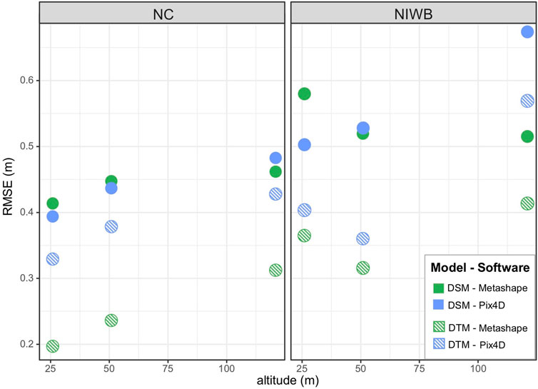
FIGURE 3. Vertical error appeared to differ across models and altitudes. Vertical error was calculated as the difference between GNSS-recorded elevations and SfM-computed model elevation at site checkpoints. Checkpoints recorded during both September (n = 46, NC, n = 64, NIWB) and February (n = 56, NC, n = 42, NIWB) were included in the RMSE.

Vertical error at checkpoints was compared across SfM-derived DTMs and available LiDAR datasets (Figure 4). Root mean square error (RMSE) are used to show agreement between computed and true data and indicate overshooting or undershooting of digitally-computed models. At NC and NIWB, computed and true elevations are well correlated using all three methods (R² = 0.64–0.84) with relatively low error (RMSE = 0.24–0.32 m). At NC, UAS-SfM processing workflows outperform LiDAR datasets in accuracy (UAS-SfM: RMSE = 0.24–0.40 m, LiDAR: RMSE = 0.64) (Figure 4). At NIWB, the LiDAR DTM yields a lower error (RMSE = 0.20 m) than either UAS-SfM software (RMSE = 0.30–0.32 m). Comparing across sites, DTM performance was similar within each UAS-SfM software, but noticeable differences in accuracy were observed using the LiDAR datasets (NC LiDAR: R² = 0.64, RMSE = 0.64 m, NIWB LiDAR: R² = 0.83, RMSE = 0.20 m).

FIGURE 4

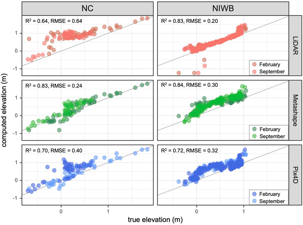
FIGURE 4. LiDAR datasets demonstrate higher vertical error than SfM-derived models at NC but lower error at NIWB. DTM vertical error is calculated as the difference between model elevation and GNSS-recorded elevations and represented for each site-method pair as the Root Mean Square Error (RMSE).

3.2 Vegetative metrics

Preliminary analyses of 3D surface models indicated that the 50 m altitude imagery represented the optimal tradeoff between model accuracy and processing time (details in Section 3.1.3). All image based vegetation metrics were calculated using models generated from 50 m altitude imagery in Pix4D only. An initial appraisal of the models generated in the two softwares indicated good agreement, so only Pix4D was used to evaluate vegetation metrics to reduce the number of variables present.

3.2.1 NDVI

The two multispectral sensors used in this analysis (MicaSense Altum and Sentera Double 4K) demonstrated different NDVI readings when flown concurrently over the same test site (Figure 5). An analysis of mean NDVI at randomly generated test plots (n = 1,000) across the marsh platform showed that NDVI readings are highly correlated between sensors (Pix4D: R² = 0.85, Metashape: R² = 0.67). However, Altum NDVI readings were greater than Sentera readings by a mean of 0.29 in Pix4D and 0.25 in Metashape. Sensor resolution and specifications potentially driving these differences are detailed in Table 1. Within sensors, reading differences across softwares may be a result of unique software workflows and processing algorithms as described in Section 2.4.

FIGURE 5

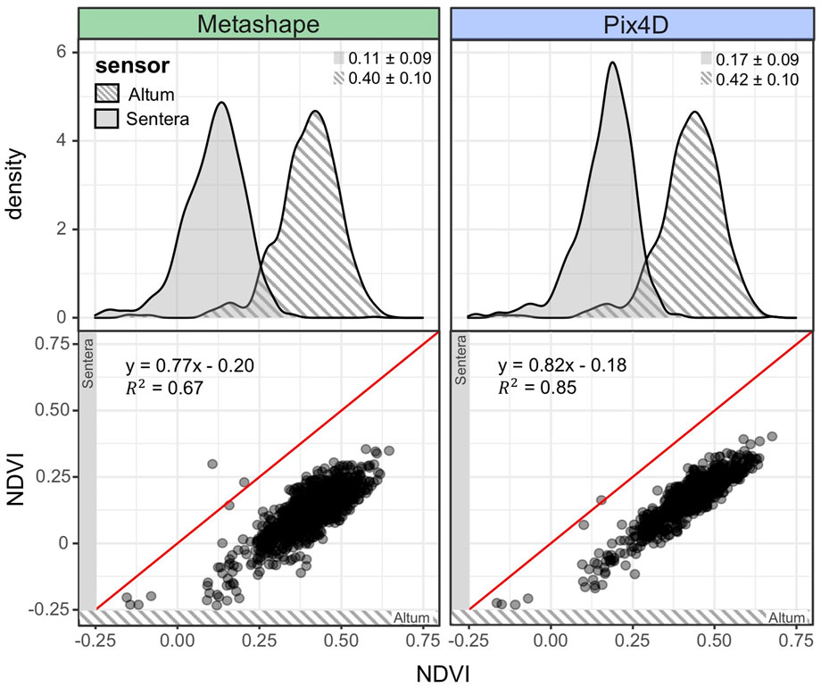
FIGURE 5. Multispectral sensors used in this analysis demonstrate different NDVI readings of the same area. Random 0.25 m² samples (n = 1,000) were generated across SfM-derived NDVI rasters and the mean NDVI value was compared across sensors and softwares.

3.2.2 Above-ground biomass

There was a strong positive correlation between SfM-computed NDVI and field-derived above ground biomass (Table 3). Imagery collected in September, when biomass was near its annual maximum, demonstrated higher computed NDVI values. February imagery, collected when standing dead vegetation was abundant, demonstrated lower computed NDVI values (Figure 6). Alternative indices derived from optical data demonstrated variable performance relative to that of NDVI. Excess Green (ExG) demonstrated a strong linear correlation with biomass at both sites (NC: R² = 0.50, NIWB: R² = 0.65) (Table 3). VIg demonstrated a weak relationship with biomass at both sites (NC: R² = 0.13, NC: R² = 0.15).

TABLE 3

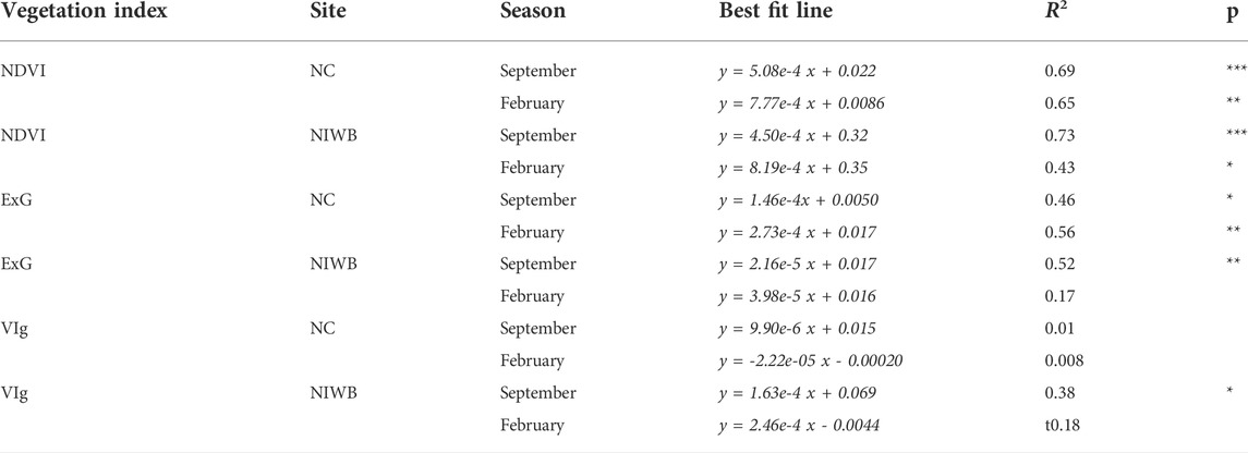
TABLE 3. Vegetation indices demonstrate significant relationships with ground-derived biomass measurements. Data represented are Pix4D-processed data using 50 m altitude flights in both February and September. ***: p < 0.001, **: p < 0.01, *: p < 0.05

FIGURE 6

FIGURE 6. Mean vegetation index values within biomass sampling plots demonstrate varying relationships with ground-derived S. alterniflora above ground biomass (AGB). Excess Green (exG) and Normalized Difference Vegetation Index (NDVI) correlate well with AGB, but these relationships vary by season (denoted by color), and Vegetation Index Green (VIg) shows no clear relationship with AGB.

3.2.3 Canopy height

Canopy height, assessed using two different methods (Eqn. 4a, 4b), is substantially underpredicted by UAS-SfM computed methods (Figure 7). At higher true stem heights, canopy height is underpredicted by greater amounts as shown by the comparison of computed data to the 1:1 line (Figure 7). At NC, there were no significant relationships between ground and computed measurements (p > 0.05) with R² values ranging from 0.08 to 0.15. At NIWB, ground-derived and UAS-SfM computed measurements were significantly correlated (p < 0.01) using all methods, with R² ranging from 0.79 to 0.85.

FIGURE 7

FIGURE 7. Computed canopy height underpredicts true canopy height. Data is visualized by season and NERRS site. Each point represents a canopy height sampling plot from which ground data (x-axis) and UAS-SfM computed data (y-axis) were extracted. Red line represents the identity line. R² is assessed for individual linear relationships. Error is computed as the Root Mean Square Error (RMSE) observed vs expected data (error as it relates to the 1:1 line) are computed to assess the goodness of fit. Subpanels represent differences between DSM and DTM values within a given digitized sampling plot (e.g. max - min: maximum DSM value - minimum DTM value).

3.2.4 Percent cover

Pixel-based percent cover estimates demonstrate difficulty assessing percent cover on the scale of ground-recorded measurements in 1 m² plots (Figure 8). Manual identification of ground and vegetated points revealed distinct NDVI signatures at NIWB in both September and February. However, NDVI signatures were mixed with overlapping ranges in both seasons at NC (Figure 8A). Thresholds developed according to Equation 5 were employed to produce computed percent cover estimates. Percent cover estimates demonstrated weak alignment with ground-recorded data at NC (Figure 8B) and no alignment with ground-recorded data at NIWB. Percent cover estimates were high at NIWB (mean = 95.05%, sd = 12.40%) despite ground estimates encompassing a wide range of values between 10 and 95%.

FIGURE 8

FIGURE 8. Percent cover estimates. (A) An NDVI threshold, denoted in red, is used to distinguish between ground and vegetation. (B) Computed percent cover estimates are compared to ground-recorded data, demonstrating weak alignment. Example sampling plots projected onto site orthomosaics are included. Points are colored by ground-recorded canopy height values within a sampling plot. Dashed lines represent the identity line.

4 Discussion

The findings of this study reveal that the quality of UAS-based mapping products can be substantially impacted by survey design. In addressing aim 1), we demonstrate that optimal GCP density and distributions can improve product georectification and UAS survey altitude impacts product resolution and surface model error. Moreover, data collection and analysis methods, which often vary across studies, can introduce variability. SfM software packages and platform-sensor combinations can have variable outputs, limiting comparability and flexibility of this approach. To address aim 2), we show that UAS hold promise for monitoring wetlands, with particular success using indexed-based proxies of above-ground biomass. In detailing UAS-SfM methods and analyzing product alignment, the results of this study lay the groundwork for a standardized methodology for UAS-SfM based monitoring of coastal wetlands.

4.1 Spatial error analyses

4.1.1 Ground control point distribution

The observed relationship between GCP density and error reinforces that increased GCP density leads to an improved ability for UAS-SfM softwares to properly georectify the orthomosaic and provide accurate ground elevation estimates (Figure 2), which has been supported by other studies (Tonkin and Midgley, 2016; Seymour et al., 2018; Villanueva and Blanco, 2019). While increasing GCPs density improves the product accuracy via georeferencing, the return on effort appears minimal at densities greater than 1 GCP/Ha (Figure 2). Studies of unvegetated habitats also show this pattern of diminishing returns in vertical accuracy at GCP densities greater than 1-2 GCP/ha (Martínez-Carricondo et al., 2018; Brunetta et al., 2021). In addition to density, this study finds that the distribution of GCPs can substantially influence vertical accuracy. Large vertical errors and high variance using “clustered” spacing highlights the importance of regularly spaced GCPs (Figure 2). This is supported by other studies which note that GCPs should stretch to the site edges to avoid tilt in the resultant elevation models (James et al., 2017), and reinforce the relationship between well-spaced GCPs and reduced model error (Tonkin and Midgley, 2016). However, in this study, both GCP distribution and density are analyzed together to provide a comprehensive recommendation for study designs. Minimal vertical errors using regularly-spaced GCPs with density 0.5 GCPs/ha or greater were observed (Figure 2), revealing a threshold that optimizes product accuracy while minimizing GCP density since each GCP requires time and effort to deploy and survey. Thus, coastal wetlands potentially do not need to be overloaded with GCPs for SfM processing if GCPs are well spaced. However, this distributional analysis also indicates that increasing the density of GCPs can reduce error to offset the impact of clustered GCPs. At many protected coastal sites it may be infeasible to regularly distribute GCPs across the study area due to inaccessibility or habitat protections. In these cases, it would be recommended to increase the number of GCPs to 2 GCP/ha or greater. NIWB NERR represented one such site, where permanent GCPs were fairly clustered along a boardwalk. High GCP densities (∼3 GCPs/ha) were used to offset errors introduced by spacing and maximize model accuracy.

4.1.2 Horizontal error

The horizontal reprojection error analysis demonstrates the tradeoff between flight altitude, with higher altitudes allowing for greater area coverage, and product resolution. Within a given UAS sensor, pixel size (GSD) increases proportionally with altitude. Across sensors, GSD differences were the result of differences in sensor resolutions (see Table 1), as GSD depends on inherent camera properties. The Mavic (NC) demonstrated higher resolution products indicated by a lower GSD as compared to the Altum (NIWB) likely due to sensor resolution differences (Table 1). The resultant GSD of Mavic flights at 50 m altitude approximately matches that of Altum flights at 25 m, indicating that users can decrease UAS flight altitude to offset reduced sensor resolutions and still achieve an optimal GSD for mapping purposes.

Horizontal error remained fairly constant across altitudes, even whilst product resolution (GSD) increased substantially (Table 2). For mapping projects, high UAS flight altitudes (>100 m) may be optimal as it allows the user to rapidly cover large areas without sacrificing much horizontal accuracy. However, the increase in GSD with altitude should be noted for projects intending to precisely map fine-scale features or boundaries. Horizontal error was generally similar (<4 cm difference) across SfM software packages, but Pix4D-generated products tended to produce smaller errors (Table 2), potentially indicating a heightened ability to georectify orthomosaics to meet ground-surveyed points. Overall, low horizontal errors (<5 cm) demonstrated by this analysis provide promising information for precise mapping of coastal and estuarine habitats, improving abilities to perform spatial analyses like the delineation of ecological boundaries and assessment of marsh retreat and advancement.

4.1.3 Vertical error

The analysis of GCP distribution at Swan Island (Section 3.1) demonstrated that with well-spaced GCPs at a density of 1 per hectare, vertical accuracies on the order of 5 cm or less are achieved on unvegetated surfaces. When vegetation is present, SfM-derived surface models represent the top of the vegetative canopy rather than the ground surface. As a result, comparisons between modeled (SfM) and measured (GNSS) elevations are influenced by the presence of vegetation. With SfM, as with LiDAR, the ability to accurately sense marsh sediment elevation is dependent upon the density of vegetative cover as this determines the number of ground hits (ie. pixels that represent sediment surface) that are sampled.

DSMs are constructed to represent the marsh canopy (i.e. plant tips) while DTMs (created by filtering the 3D point cloud to remove all points above the ground surface) represent bare-earth models intended to exclude vegetation and other structures. Because these sites are vegetated ecosystems, it is expected that GNSS-recorded, “true” values represent bare-earth elevation and therefore should closely align with DTM-derived elevations. Anders et al. (2019) assessed Agisoft Metashape-generated (formerly Agisoft Photoscan) DTMs over shrubland habitat which yielded an RMSE of 0.5m, similar to the values observed in this study (Figure 3) (Anders et al., 2019). However, the range of RMSE values for both surface and terrain models demonstrate the challenges with accurately measuring vegetation height from imagery. With S. alterniflora stems ranging from approximately 0–2 m tall, high error in elevation models means that, proportionally, much of the plant stem may be missed in calculations.

Comparing error across softwares, the notable differences in DTM error is potentially a result of dissimilarity in DTM construction methods across softwares. Metashape allows for more user input in the DTM construction, permitting the user to define the maximum angle and distance between points to filter the DSM in the creation of a DTM (Agisoft Metashape User Manual - Professional Edition, Version 1.5). In contrast, Pix4D does not allow these parameters to be defined (Pix4D, 2022). Because of these differences, the DTMs do not appear to be comparable across softwares. The DSMs contain higher RMSE than DTMs but are more consistent when comparing across softwares (Figure 3) presumably due to software similarities in DSM construction methods.

Analyzing altitudinal trends, the increase in vertical error observed at higher altitudes speaks to the tradeoff between efficiency (higher altitude flights cover a larger area in fewer images) and precision (Figure 3, Supplementary Figure S1). For this study, 50 m was chosen as the optimal flight altitude based on Figure 3, as it minimizes DSM RMSE at NIWB, only shows a slight increase in error from 25 m altitude at NC, and is the most consistent across softwares. While there is a clear tradeoff in product resolution with flight altitude (see Table 2), vertical accuracy does not demonstrate a clear trend with altitude. A similar study using a consumer-grade UAS to survey a shrubland area revealed an increase in vertical error with altitude (altitude range: 126–235 m) at the first site and consistent vertical error across altitudes at the second site (Anders et al., 2020). The range of low altitudes (25–120 m) used in this study are those most commonly used by United States UAS pilots given that flight altitudes above 120 m are restricted by the Federal Aviation Administration (FAA). In analyzing product accuracy over this relevant altitudinal range, this study may inform flight planning for efficient mapping of coastal vegetated areas.

UAS-SfM-derived DTM errors are similar to that of other studies of similar habitats (Yanagi and Chikatsu, 2016; Goodbody et al., 2018). For example, Goodbody et al. (2018), using a fixed-wing UAS to construct DTMs of vegetated habitats, reported an average of 0–0.5 m error in shrubland habitats. UAS-SfM DTM error in similar short vegetation in this study is comparable (RMSE: 0.24–0.32 m; Figure 4). Comparing the two UAS-SfM methods to LiDAR data, it is clear that LiDAR datasets, though substantially lower in resolution and lacking real-time observations, yield comparable elevation estimates to UAS-SfM-constructed bare-earth models. This observation, which is supported by other studies, may be due to the high-accuracy positioning of aircraft hosting LiDAR sensors (Dayamit et al., 2015; DiGiacomo et al., 2020). Comparing all three methods, Metashape-generated DTMs align best with GNSS-recorded values with high R² values and low RMSE estimates (Figure 4). This may be explained by noting that Metashape DTM-generation, discussed in Section 2.4, allows for a high level of user input.

4.2 Vegetation metrics

4.2.1 NDVI

The observed differences in NDVI readings across sensors indicate that raw NDVI values cannot be compared across the two sites (Figure 5). With an observed difference in NDVI readings between sensors of approximately 0.3 across the biomass values observed in this study, it is clear that absolute NDVI values cannot be compared across sensors, even when flying the same site under the same conditions. For comparative work (i.e. observing changes in marsh biomass over time), it is therefore recommended that the same sensor is used. However, this may become difficult as sensors improve and change over time. For this reason, test flights of the same area under the same conditions may be flown to develop a transformation between sensors and enable direct comparisons of NDVI values. Sensor-specific differences in NDVI values have been outlined across different satellite-derived datasets and between UAS and satellite data and attributed to differences in bandwidths, spatial resolutions, and data processing (Huang et al., 2021). One important distinction is that multispectral data from the Micansense Altum (NIWB) sensor is radiometrically calibrated using a calibration panel while that of the Sentera Double 4K (NC) is non-calibrated. Radiometric calibration, which converts the sensor radiance into reflectance values and accounts for changes in ambient light, works to provide standardized data that is more comparable across conditions (Lu, 2006). While this adds greater consistency and reliability to the Altum dataset, it has been noted that the factory-provided calibration of commercial-grade UAS with multispectral capabilities can be limited and fail to account for sensor changes and deterioration over time (Mamaghani and Salvaggio, 2019). Alternative calibration methods have been developed to improve accuracy across flights, but these methods may require additional time and specialized knowledge (Mamaghani and Salvaggio, 2019).

4.2.2 above-ground biomass

NDVI is recommended as the most reliable option as it has the strongest relationship with biomass (R² = 0.42–0.73, Table 3) and is significantly linearly correlated with biomass across sites and seasons. Moreover, these linear relationships (slopes, intercepts) are consistent across seasons at each site (Table 3). This indicates the potential to use a linear model to accurately predict biomass changes over time at a given site from UAS imagery. Previous studies of S. alterniflora biomass using SPOT6 satellite remote sensing images and airborne hyperspectral scanners report a similar relationship with NDVI (R² = 0.499, R² = 0.635, respectively) (Wang et al., 2017; Zhou et al., 2018). Several UAS-based studies have shown clear linear relationships between biomass and NDVI readings in coastal wetlands (Zhou et al., 2018; Doughty and Cavanaugh, 2019). This study supports the ability of UAS-based multispectral imagery to provide non-invasive estimates of wetland biomass across multiple sites and seasons.

Indices that rely on optical data alone, like ExG and VIg, provide a clear advantage in that these data are more accessible and generally less expensive. ExG also demonstrates a strong relationship with biomass (R² = 0.17–0.56, Table 3), although the strength of this relationship is variable across seasons (Figure 6). In the absence of multispectral data, ExG may provide reliable estimates during peak biomass that don’t require advanced multispectral sensors or calibrations. While VIg largely fails to capture changes in biomass in this study, it is possible that VIg may perform well in other systems. This is supported by other work showing that VIg is tightly correlated to biomass in studies using commercial-grade UAS to survey maize fields (R² = 0.68) (Niu et al., 2019) and hyperspectral UAS to study changes in summer barley biomass (R² = 0.62) (Bendig et al., 2015). While these represent several common vegetation indices, future work may explore the potential of more complex indices, or combinations of indices, which have been shown in certain studies to improve predictions of AGB (Huete, 1988; Qi et al., 1994; Fuentes-Peailillo et al., 2018; Poley and McDermid, 2020).

Relationships with biomass should be further analyzed with an understanding that many current vegetation characteristics are designed for allometric-based estimates of above-ground biomass. Traditional approaches involve clipping plants, like the ground-based data in this study, to assess biomass. Even non-invasive approaches, like measuring density and stem height as a proxy for biomass, require substantial effort and result in sparse data points across a dynamic habitat. Furthermore, in many coastal marshes the sediments of the lower elevations are so unconsolidated as to make access for ground-based measurements impractical or simply too physically destructive to warrant repeat sampling. The ability to estimate AGB using image-based indices across landscapes transforms the scale at which we can monitor these ecosystems. Moreover, the consistency across seasonal endpoints (dormant season and peak-biomass) demonstrated by linear models (Table 3) indicates potential to accurately monitor biomass within a given site. In this way, UAS may be used to rapidly and efficiently collect vegetation data over time, allowing researchers and managers to estimate biomass across meaningful spatiotemporal scales.

4.2.3 Canopy height

All canopy height estimation methods employed here indicate that canopy height is substantially underestimated by UAS-derived heights and that UAS-SfM methods underestimate plant height more at higher stem heights (Figure 7). This trend, observed in previous studies of S. alterniflora structure, has been addressed in other studies by inflating UAS-SfM computed plant heights to improve the accuracy of canopy height estimates (DiGiacomo et al., 2020). Because the purpose of this study is to understand the feasibility of the SfM software user to produce canopy height estimates from UAS-SfM products, a transformation was not employed and only raw values were analyzed. The finding that canopy height underprediction increases with stem height is likely due to the fact that taller S. alterniflora plants tend to bend more under their own weight and the outer leaves of tall plants often drape outward from the main stem, whereas shorter plants tend be more compact and erect. The results of the current investigation indicate that canopy height estimate accuracy is variable across sites and seasons. Site-based differences may be explained by the fact that the two sites represent different ranges of canopy heights, with NIWB generally representing taller plants (mean ± sd: 1.26 ± 0.45 m) and NC representing shorter plants (0.81 ± 0.49 m). While short plants (0–0.5 m) appear to fall close to the 1:1 line with low error (RMSE: 0.22–0.23 m), deviation from the 1:1 line becomes more pronounced with canopy height (Figure 7). Tall plants (height >0.5 m) observed at both sites and seasons have large errors (RMSE: 0.95–1.09 m). Seasonal differences in canopy height estimation accuracy may be explained by this height-driven error, as plant height tends to be reduced in the dormant season. Methodological differences for height measurements across seasons (see Section 2.5), however, may also impact this relationship as stem straight-line length was measured in the peak-biomass data, while sloped stem height was measured in the dormant season. While we might therefore expect to observe more underestimation in plant height by UAS in the September data, which is observed at NC (Figure 7), it is difficult to tease apart whether methodological differences or true seasonal differences in plant height (i.e. senescence) drive these observed differences. We believe that this highlights the need to re-evaluate and standardize field practices for canopy height measurements. While it is typical to use straight-line stem height as “true” canopy height in manual vegetation height field studies, remotely sensed measurements record natural, or sloped, canopy height (Currin et al., 2008; DiGiacomo et al., 2020). However, in the dormant season, when the same ground-based methods were employed across sites, a better fit was still observed at NC (Figure 7). This may be explained by lower vertical error in NC DSM and DTM products (Figure 3) or the previously mentioned difference in ranges of canopy heights across sites. Future studies might better resolve this trend by targeting field sites with a wider range of stem heights to reduce the number of variables potentially impacting metrics of canopy height error. Additionally, as canopy height may vary within a 1 m² area, we suggest that future work decrease the plot size within which ground-based measurements of stem height are recorded.

4.2.4 Percent cover

The NDVI signatures of ground and vegetation at NC show considerable overlap, indicating a difficulty to separate ground from vegetation using a fixed NDVI threshold at NC (Figure 8A). In contrast, the distinct NDVI signatures observed at NIWB (Figure 8A) may provide evidence for the possibility of NDVI-based thresholding to separate ground and vegetation pixels for percent cover estimates. However, as can be seen in Figure 8B, this thresholding approach does not produce percent cover values aligned with ground-recorded estimates. The failure of a pixel-based percent cover approach to align with field-recorded values may be a result of an oversaturation of NDVI. Spectral indices such as NDVI can present a saturation problem, where indices plateau at a threshold where the index is fully saturated, typically an issue in areas characterized by densely vegetated canopies (Asner et al., 2003; Lu, 2006; Zhao et al., 2016). As a result, changes in cover beyond these thresholds cannot be isolated. With taller plants at NIWB, and therefore greater leaf area, computed percent cover estimates appear to become saturated with all image-based estimates nearing 100% cover (Figure 8B). These tall plants (>1.0 m) are associated with high percent cover estimates (mean ± sd: 84.38 ± 24.26%), while short plants (defined as < 0.5 m), that characterize NC are associated with lower computed percent cover estimates (mean = 20.17%, sd = 35.78%). Therefore, beyond canopy density, as outlined in previous studies (Lu, 2006; Zhou et al., 2018), plant height may influence aerial multispectral estimates of percent cover given that there is greater leaf area. It is also possible that, given the resolution of the sensors, percent cover may not be feasible to extract on this scale. Classification of wetland imagery and the development of percent cover estimates has been executed using UAS-based approaches at larger scales, such as Chabot and Bird (2013), who used 25 m radius circular plots to successfully assess percent cover (Chabot and Bird, 2013).

Though, in this study, ground-based estimates of percent cover are considered to be “true” data, it should be noted that these manual estimates vary in methodology and may be inconsistent. Differences in percent cover ground data collection methods at NC and NIWB may be a source of variability in the data. The point-intercept method used at NC may be more objective, as it has rigorous quantitative metrics for computing cover (see Section 2.5), which may help to explain the increased alignment of UAS and ground data at NC (Figure 8A). Ground-based methods for assessing percent cover may be limited by the horizontal frame of reference and impacted by canopy height, density, and vegetation type. For these reasons, aerial estimates may be less subjective than ground-based estimates and provide more consistent, reliable estimations of vegetation cover.

5 Conclusion

Inexpensive, widely available UAS platforms provide a valuable tool for habitat monitoring and change detection in coastal ecosystems. We demonstrate that mapping product accuracy is impacted by GCP density and distribution as well as common UAS operational parameters. With adequate attention to flight planning and SfM processing routines, UAS can be used to estimate plant biomass and create marsh surface models that are comparable in accuracy to manually-derived products. The consistently low error in XY position associated with UAS-SfM models suggests that these products will also be of great value for measuring elevation change and structural metrics over time in the face of rapid change in coastal and estuarine habitats. In describing the variability and tradeoffs associated with UAS-based mapping operations and parameters, this study helps to increase transparency and comparability of UAS-SfM based monitoring and assessment of coastal wetlands. The results of this work will expand our ability to accurately and rapidly assess and monitor coastal wetlands on unprecedented scales, a critical step forward in light of recent coastal change and restoration efforts.

Data availability statement

The datasets presented in this study can be found in online repositories. The names of the repository/repositories and accession number(s) can be found below: https://doi.org/10.7924/r4sb46t2c.

Author contributions

Conceptualization, JD, JR, ES, and BP; methodology, AD, RG, JD, JR, BP, and ES; software, AD and RG; validation, AD and RG; formal analysis, AD and RG; investigation, BP and ES; resources, BP, ES, JD, and JR; data curation, AD and RG; writing—original draft preparation, AD; writing—review and editing, AD, JD, JR, BP, ES, and RG; visualization, AD; supervision, JD and JR; project administration, JD, JR, ES, and BP; funding acquisition, JD JR, ES, and BP. All authors have read and agreed to the published version of the manuscript.

Funding

This work was made possible by a grant from the NOAA Office of Oceanic and Atmospheric Research (Grant #W8KSCXR).

Acknowledgments

The authors would like to thank Bryan Costa and Leanne Poussard of NCCOS for preliminary reviews of this manuscript. Brittany Morse of NI-WB NERR and Charlie Deaton of NCNERR supported field sampling and image acquisition. Chris Kinkade of the National Estuarine Research Reserve program played a pivotal role in project administration and outreach.

Conflict of interest

RG was employed by Consolidated Safety Services Inc, for National Oceanic and Atmospheric Administration.

The remaining authors declare that the research was conducted in the absence of any commercial or financial relationships that could be construed as a potential conflict of interest.

Publisher’s note

All claims expressed in this article are solely those of the authors and do not necessarily represent those of their affiliated organizations, or those of the publisher, the editors and the reviewers. Any product that may be evaluated in this article, or claim that may be made by its manufacturer, is not guaranteed or endorsed by the publisher.

Supplementary material

The Supplementary Material for this article can be found online at: https://www.frontiersin.org/articles/10.3389/frsen.2022.924969/full#supplementary-material

References

Adam, E., Mutanga, O., and Rugege, D. (2010). Multispectral and hyperspectral remote sensing for identification and mapping of wetland vegetation: A review. Wetl. Ecol. Manag. 18, 281–296. doi:10.1007/s11273-009-9169-z

CrossRef Full Text | Google Scholar

Agisoft LLC (2021). Agisoft metashape user manual—professional edition. Version 1.7 Available at: https://www.agisoft.com/metashape-pro_1_7_en (Accessed January 1, 2021).

Google Scholar

Altum and MicaSense (2021). Altum | MicaSense. Available at: https://micasense.com/altum/(Accessed May 12, 2021).

Google Scholar

Anders, N., Smith, M., Suomalainen, J., Cammeraat, E., Valente, J., and Keesstra, S. (2020). Impact of flight altitude and cover orientation on Digital Surface Model (DSM) accuracy for flood damage assessment in Murcia (Spain) using a fixed-wing UAV. Earth Sci. Inf. 13, 391–404. doi:10.1007/s12145-019-00427-7

CrossRef Full Text | Google Scholar

Anders, N., Valente, J., Masselink, R., and Keesstra, S. (2019). Comparing filtering techniques for removing vegetation from UAV-based photogrammetric point clouds. Drones 3, 61. doi:10.3390/drones3030061

CrossRef Full Text | Google Scholar

Asner, G. P., Scurlock, J. M. O., and Hicke, J. A. (2003). Global synthesis of leaf area index observations: Implications for ecological and remote sensing studies. Glob. Ecol. Biogeogr. 12, 191–205. doi:10.1046/j.1466-822X.2003.00026.x

CrossRef Full Text | Google Scholar

Barbier, E. B., Hacker, S. D., Kennedy, C., Koch, E. W., Stier, A. C., and Silliman, B. R. (2011). The value of estuarine and coastal ecosystem services. Ecol. Monogr. 81, 169–193. doi:10.1890/10-1510.1

CrossRef Full Text | Google Scholar

Barnas, A. F., Chabot, D., Hodgson, A. J., Johnston, D. W., Bird, D. M., and Ellis-Felege, S. N. (2020). A standardized protocol for reporting methods when using drones for wildlife research. J. Unmanned Veh. Syst. 8, 89–98. doi:10.1139/juvs-2019-0011

CrossRef Full Text | Google Scholar

Bendig, J., Yu, K., Aasen, H., Bolten, A., Bennertz, S., Broscheit, J., et al. (2015). Combining UAV-based plant height from crop surface models, visible, and near infrared vegetation indices for biomass monitoring in barley. Int. J. Appl. Earth Obs. Geoinf. 39, 79–87. doi:10.1016/j.jag.2015.02.012

CrossRef Full Text | Google Scholar

Brunetta, R., Duo, E., and Ciavola, P. (2021). Evaluating short-term tidal flat evolution through uav surveys: A case study in the Po delta (Italy). Remote Sens. (Basel). 13, 2322. doi:10.3390/rs13122322

CrossRef Full Text | Google Scholar

Chabot, D., and Bird, D. M. (2013). Small unmanned aircraft: Precise and convenient new tools for surveying wetlands. J. Unmanned Veh. Syst. 01, 15–24. doi:10.1139/juvs-2013-0014

CrossRef Full Text | Google Scholar

Chen, Y., Dong, J., Xiao, X., Zhang, M., Tian, B., Zhou, Y., et al. (2016). Land claim and loss of tidal flats in the Yangtze Estuary. Sci. Rep. 6, 24018. doi:10.1038/srep24018

PubMed Abstract | CrossRef Full Text | Google Scholar

Currin, C. A., Delano, P. C., and Valdes-Weaver, L. M. (2008). Utilization of a citizen monitoring protocol to assess the structure and function of natural and stabilized fringing salt marshes in North Carolina. Wetl. Ecol. Manag. 16, 97–118. doi:10.1007/s11273-007-9059-1

CrossRef Full Text | Google Scholar

Dayamit, O. M., Pedro, M. F., Ernesto, R. R., and Fernando, B. L. (2015). “Digital elevation model from non-metric camera in UAS compared with lidar technology,” in International Conference on Unmanned Aerial Vehicles in Geomatics, Toronto, Canada. The International Archives of the Photogrammetry, Remote Sensing and Spatial Information Sciences XL-1/W4, 411–414. doi:10.5194/isprsarchives-XL-1-W4-411-2015

CrossRef Full Text | Google Scholar

DiGiacomo, A. E., Bird, C. N., Pan, V. G., Dobroski, K., Atkins-Davis, C., Johnston, D. W., et al. (2020). Modeling salt marsh vegetation height using unoccupied aircraft systems and structure from motion. Remote Sens. (Basel). 12, 2333. doi:10.3390/rs12142333

CrossRef Full Text | Google Scholar

Double 4K Sensor - Sentera (2021). Sentera Double 4K sensor | Sentera | red edge Sentera. Available at: https://sentera.com/product/double-4k-sensor/(Accessed May 12, 2021).

Google Scholar

Doughty, C. L., and Cavanaugh, K. C. (2019). Mapping coastal wetland biomass from high resolution unmanned aerial vehicle (UAV) imagery. Remote Sens. (Basel). 11, 540. doi:10.3390/rs11050540

CrossRef Full Text | Google Scholar

Farris, A. S., Defne, Z., and Ganju, N. K. (2019). Identifying salt marsh shorelines from remotely sensed elevation data and imagery. Remote Sens. (Basel). 11, 1795. doi:10.3390/rs11151795

CrossRef Full Text | Google Scholar

Fennessy, M. S., Jacobs, A. D., and Kentula, M. E. (2007). An evaluation of rapid methods for assessing the ecological condition of wetlands. Wetlands 27, 543–560. doi:10.1672/0277-5212(2007)27[543:AEORMF]2.0.CO;2

CrossRef Full Text | Google Scholar

Fraser, B. T., and Congalton, R. G. (2018). Issues in unmanned aerial systems (UAS) data collection of complex forest environments. Remote Sens. (Basel). 10, 908. doi:10.3390/rs10060908

CrossRef Full Text | Google Scholar

Fuentes-Peailillo, F., Ortega-Farías, S., Rivera, M., Bardeen, M., and Moreno, M. (2018). “Comparison of vegetation indices acquired from RGB and Multispectral sensors placed on UAV,” in Proceedings of the 2018 IEEE International Conference on Automation/XXIII Congress of the Chilean Association of Automatic Control (ICA-ACCA), Concepcion, Chile, October 17–19, 2018, 1–6. doi:10.1109/ICA-ACCA.2018.8609861

CrossRef Full Text | Google Scholar

Goodbody, T. R. H., Coops, N. C., Hermosilla, T., Tompalski, P., and Pelletier, G. (2018). Vegetation phenology driving error variation in digital aerial photogrammetrically derived terrain models. Remote Sens. (Basel). 10, 1554. doi:10.3390/rs10101554

CrossRef Full Text | Google Scholar

Green, E. P., Mumby, P. J., Edwards, A. J., and Clark, C. D. (1996). A review of remote sensing for the assessment and management of tropical coastal resources. Coast. Manage. 24, 1–40. doi:10.1080/08920759609362279

CrossRef Full Text | Google Scholar

Haskins, J., Endris, C., Thomsen, A. S., Gerbl, F., Fountain, M. C., and Wasson, K. (2021). UAV to inform restoration: A case study from a California tidal marsh. Front. Environ. Sci. 9, 642906. doi:10.3389/fenvs.2021.642906

CrossRef Full Text | Google Scholar

Huang, S., Tang, L., Hupy, J. P., Wang, Y., and Shao, G. (2021). A commentary review on the use of normalized difference vegetation index (NDVI) in the era of popular remote sensing. J. For. Res. 32, 1–6. doi:10.1007/s11676-020-01155-1

CrossRef Full Text | Google Scholar

Huete, A. R. (1988). A soil-adjusted vegetation index (SAVI). Remote Sens. Environ. 25, 295–309. doi:10.1016/0034-4257(88)90106-X

CrossRef Full Text | Google Scholar

Jackson, J. B. C., Kirby, M. X., Berger, W. H., Bjorndal, K. A., Botsford, L. W., Bourque, B. J., et al. (2001). Historical overfishing and the recent collapse of coastal ecosystems. Science 293, 629–637. doi:10.1126/science.1059199

PubMed Abstract | CrossRef Full Text | Google Scholar

James, M. R., Robson, S., d’Oleire-Oltmanns, S., and Niethammer, U. (2017). Optimising UAV topographic surveys processed with structure-from-motion: Ground control quality, quantity and bundle adjustment. Geomorphology 280, 51–66. doi:10.1016/j.geomorph.2016.11.021

CrossRef Full Text | Google Scholar

James-Pirri, M.-J., Roman, C. T., and Erwin, R. M. (2002). Field methods manual: US fish and wildlife service (region 5) salt marsh study Narragansett, RI: University of Rhode Island.

Google Scholar

Kameyama, S., and Sugiura, K. (2021). Effects of differences in structure from motion software on image processing of unmanned aerial vehicle photography and estimation of crown area and tree height in forests. Remote Sens. (Basel). 13, 626. doi:10.3390/rs13040626

CrossRef Full Text | Google Scholar

Klemas, V. (2013). Remote sensing of coastal wetland biomass: An overview. J. Coast. Res. 29, 1016–1028. doi:10.2112/JCOASTRES-D-12-00237.1

CrossRef Full Text | Google Scholar

Laengner, M. L., Siteur, K., and van der Wal, D. (2019). Trends in the seaward extent of saltmarshes across europe from long-term satellite data. Remote Sens. (Basel). 11, 1653. doi:10.3390/rs11141653

CrossRef Full Text | Google Scholar

Lopes, C. L., Mendes, R., Caçador, I., and Dias, J. M. (2020). Assessing salt marsh extent and condition changes with 35 years of Landsat imagery: Tagus Estuary case study. Remote Sens. Environ. 247, 111939. doi:10.1016/j.rse.2020.111939

CrossRef Full Text | Google Scholar

Lotze, H. K., Lenihan, H. S., Bourque, B. J., Bradbury, R. H., Cooke, R. G., Kay, M. C., et al. (2006). Depletion, degradation, and recovery potential of estuaries and coastal seas. Science 312, 1806–1809. doi:10.1126/science.1128035

PubMed Abstract | CrossRef Full Text | Google Scholar

Lu, D. (2006). The potential and challenge of remote sensing-based biomass estimation. Int. J. Remote Sens. 27, 1297–1328. doi:10.1080/01431160500486732

CrossRef Full Text | Google Scholar

MacKay, H., Finlayson, C. M., Fernández-Prieto, D., Davidson, N., Pritchard, D., and Rebelo, L.-M. (2009). The role of earth observation (EO) technologies in supporting implementation of the ramsar convention on wetlands. J. Environ. Manage. 90, 2234–2242. doi:10.1016/j.jenvman.2008.01.019

PubMed Abstract | CrossRef Full Text | Google Scholar

Mamaghani, B., and Salvaggio, C. (2019). Multispectral sensor calibration and characterization for sUAS remote sensing. Sensors 19, 4453. doi:10.3390/s19204453

PubMed Abstract | CrossRef Full Text | Google Scholar

Martínez-Carricondo, P., Agüera-Vega, F., Carvajal-Ramírez, F., Mesas-Carrascosa, F.-J., García-Ferrer, A., and Pérez-Porras, F.-J. (2018). Assessment of UAV-photogrammetric mapping accuracy based on variation of ground control points. Int. J. Appl. Earth Obs. Geoinf. 72, 1–10. doi:10.1016/j.jag.2018.05.015

CrossRef Full Text | Google Scholar

Mavic 2 (2021). Mavic 2 - product information - DJI DJI off. Available at: https://www.dji.com/mavic-2/info (Accessed May 12, 2021).

Google Scholar

McCarthy, M. J., Colna, K. E., El-Mezayen, M. M., Laureano-Rosario, A. E., Méndez-Lázaro, P., Otis, D. B., et al. (2017). Satellite remote sensing for coastal management: A review of successful applications. Environ. Manage. 60, 323–339. doi:10.1007/s00267-017-0880-x

PubMed Abstract | CrossRef Full Text | Google Scholar

Meixler, M. S., Kennish, M. J., and Crowley, K. F. (2018). Assessment of plant community characteristics in natural and human-altered coastal marsh ecosystems. Estuaries Coast. 41, 52–64. doi:10.1007/s12237-017-0296-0

CrossRef Full Text | Google Scholar

Meyer, G. E., and Neto, J. C. (2008). Verification of color vegetation indices for automated crop imaging applications. Comput. Electron. Agric. 63, 282–293. doi:10.1016/j.compag.2008.03.009

CrossRef Full Text | Google Scholar

Minchinton, T. E., Shuttleworth, H. T., Lathlean, J. A., McWilliam, R. A., and Daly, T. J. (2019). Impacts of cattle on the vegetation structure of mangroves. Wetlands 39, 1119–1127. doi:10.1007/s13157-019-01143-0

CrossRef Full Text | Google Scholar

Morris, J. T., Sundareshwar, P. V., Nietch, C. T., Kjerfve, B., and Cahoon, D. R. (2002). Responses of coastal wetlands to rising sea level. Ecology 83, 2869–2877. doi:10.1890/0012-9658(2002)083[2869:ROCWTR]2.0.CO;2

CrossRef Full Text | Google Scholar

National Estuarine Research Reserve System (2021). National estuarine research Reserve system. Available at: https://coast.noaa.gov/nerrs/about/(Accessed May 3, 2021).

Google Scholar

Niu, Y., Zhang, L., Zhang, H., Han, W., and Peng, X. (2019). Estimating above-ground biomass of maize using features derived from UAV-based RGB imagery. Remote Sens. (Basel). 11, 1261. doi:10.3390/rs11111261

CrossRef Full Text | Google Scholar

NOAA (2021). NOAA: Data access viewer. Available at: https://coast.noaa.gov/dataviewer/(Accessed July 14, 2021).

Google Scholar

Noss, R. F., Platt, W. J., Sorrie, B. A., Weakley, A. S., Means, D. B., Costanza, J., et al. (2015). How global biodiversity hotspots may go unrecognized: Lessons from the North American coastal plain. Divers. Distrib. 21, 236–244. doi:10.1111/ddi.12278

CrossRef Full Text | Google Scholar

OCM Partners (2017). 2017 SC DNR lidar DEM: Georgetown county. Available at: https://www.fisheries.noaa.gov/inport/item/57134 (Accessed September 1, 2021).

Google Scholar

OCM Partners (2018). 2018 USACE NCMP post-florence Topobathy lidar DEM: Southeast coast (VA, NC, SC). Available at: https://www.fisheries.noaa.gov/inport/item/57345 (Accessed September 1, 2021).

Google Scholar

Peterson, P. M., Romaschenko, K., Arrieta, Y. H., and Saarela, J. M. (2014). A molecular phylogeny and new subgeneric classification of Sporobolus (Poaceae: Chloridoideae: Sporobolinae). Taxon 63, 1212–1243. doi:10.12705/636.19

CrossRef Full Text | Google Scholar

Pettorelli, N., Bühne, H. S., Tulloch, A., Dubois, G., Macinnis-Ng, C., Queirós, A. M., et al. (2018). Satellite remote sensing of ecosystem functions: Opportunities, challenges and way forward. Remote Sens. Ecol. Conserv. 4, 71–93. doi:10.1002/rse2.59

CrossRef Full Text | Google Scholar

Pham, T. D., Xia, J., Ha, N. T., Bui, D. T., Le, N. N., and Tekeuchi, W. (2019). A review of remote sensing approaches for monitoring Blue carbon ecosystems: Mangroves, seagrassesand salt marshes during 2010–2018. Sensors 19, 1933. doi:10.3390/s19081933

CrossRef Full Text | Google Scholar

Pix4D (2022). Pix4D manual – support. Available at: https://support.pix4d.com/hc/en-us/sections/360003718992-Manual (Accessed April 7, 2022).

Google Scholar

Poley, L. G., and McDermid, G. J. (2020). A systematic review of the factors influencing the estimation of vegetation aboveground biomass using unmanned aerial systems. Remote Sens. (Basel). 12, 1052. doi:10.3390/rs12071052

CrossRef Full Text | Google Scholar

Psuty, N. P., Ames, K., Habeck, A., and Schmelz, W. (2018). Responding to coastal change: Creation of a regional approach to monitoring and management, northeastern region, U.S.A. Ocean. Coast. Manag. 156, 170–182. doi:10.1016/j.ocecoaman.2017.08.004

CrossRef Full Text | Google Scholar

Qi, J., Chehbouni, A., Huete, A. R., Kerr, Y. H., and Sorooshian, S. (1994). A modified soil adjusted vegetation index. Remote Sens. Environ. 48, 119–126. doi:10.1016/0034-4257(94)90134-1

CrossRef Full Text | Google Scholar

Roman, C. T., James-Pirri, , Mary-Jane, M.-J., and Heltshe, J. F. (2001). Monitoring salt marsh vegetation: A protocol for the long-term coastal ecosystem monitoring program at cape cod national seashore. Narragansett, RI: USGS Patuxent Wildl. Res. Cent. Coast. Res. Field Stn. Univ. R. I., 55.

Google Scholar

Roughgarden, J., Running, S. W., and Matson, P. A. (1991). What Does Remote Sensing Do For Ecology? Ecology 72, 1918–1922. doi:10.2307/1941546

CrossRef Full Text | Google Scholar

Seymour, A. C., Ridge, J. T., Rodriguez, A. B., Newton, E., Dale, J., and Johnston, D. W. (2018). Deploying Fixed Wing Unoccupied Aerial Systems (UAS) for Coastal Morphology Assessment and Management. J. Coast. Res. 34, 704. doi:10.2112/jcoastres-d-17-00088.1

CrossRef Full Text | Google Scholar

Sona, G., Pinto, L., Pagliari, D., Passoni, D., and Gini, R. (2014). Experimental analysis of different software packages for orientation and digital surface modelling from UAV images. Earth Sci. Inf. 7, 97–107. doi:10.1007/s12145-013-0142-2

CrossRef Full Text | Google Scholar

Spalding, M. D., Ruffo, S., Lacambra, C., Meliane, I., Hale, L. Z., Shepard, C. C., et al. (2014). The role of ecosystems in coastal protection: Adapting to climate change and coastal hazards. Ocean. Coast. Manag. 90, 50–57. doi:10.1016/j.ocecoaman.2013.09.007

CrossRef Full Text | Google Scholar

Thomsen, A. S., Krause, J., Appiano, M., Tanner, K. E., Endris, C., Haskins, J., et al. (2021). Monitoring Vegetation Dynamics at a Tidal Marsh Restoration Site: Integrating Field Methods, Remote Sensing and Modeling. Estuaries Coast. 45, 523–538. doi:10.1007/s12237-021-00977-4

CrossRef Full Text | Google Scholar

Tonkin, T. N., and Midgley, N. G. (2016). Ground-Control Networks for Image Based Surface Reconstruction: An Investigation of Optimum Survey Designs Using UAV Derived Imagery and Structure-from-Motion Photogrammetry. Remote Sens. (Basel). 8, 786. doi:10.3390/rs8090786

CrossRef Full Text | Google Scholar

Trueblood, D., Almazán-Casali, S., Arnott, J., Brass, M., Lemos, M. C., Matso, K., et al. (2019). Advancing Knowledge for Use in Coastal and Estuarine Management: Competitive Research in the National Estuarine Research Reserve System. Coast. Manage. 47, 337–346. doi:10.1080/08920753.2019.1598221

CrossRef Full Text | Google Scholar

Villanueva, J. K. S., and Blanco, A. C. (2019). Optimization Of Ground Control Point (GCP) Configuration For Unmanned Aerial Vehicle (UAV) Survey Using Structure From Motion (SFM). Int. Arch. Photogramm. Remote Sens. Spat. Inf. Sci. XLII-4/W12, 167–174. doi:10.5194/isprs-archives-XLII-4-W12-167-2019

CrossRef Full Text | Google Scholar

Wang, J., Liu, Z., Yu, H., and Li, F. (2017). Mapping Spartina alterniflora Biomass Using LiDAR and Hyperspectral Data. Remote Sens. (Basel). 9, 589. doi:10.3390/rs9060589

CrossRef Full Text | Google Scholar

Whitehead, K., and Hugenholtz, C. (2014). Remote sensing of the environment with small unmanned aircraft systems (UASs), part 1: a review of progress and challenges. J. Unmanned Veh. Syst. 02, 69–85. doi:10.1139/juvs-2014-0006

CrossRef Full Text | Google Scholar

Yanagi, H., and Chikatsu, H. (2016). Performance Evaluation of 3d Modeling Software for Uav Photogrammetry. Int. Arch. Photogramm. Remote Sens. Spat. Inf. Sci. 41, 147–152. doi:10.5194/isprs-archives-XLI-B5-147-2016

CrossRef Full Text | Google Scholar

Zhao, P., Lu, D., Wang, G., Wu, C., Huang, Y., and Yu, S. (2016). Examining Spectral Reflectance Saturation in Landsat Imagery and Corresponding Solutions to Improve Forest Aboveground Biomass Estimation. Remote Sens. (Basel). 8, 469. doi:10.3390/rs8060469

CrossRef Full Text | Google Scholar

Zhou, Z., Yang, Y., and Chen, B. (2018). Estimating Spartina alterniflora fractional vegetation cover and aboveground biomass in a coastal wetland using SPOT6 satellite and UAV data. Aquat. Bot. 144, 38–45. doi:10.1016/j.aquabot.2017.10.004

CrossRef Full Text | Google Scholar