Spatiotemporal change analysis for snowmelt over the Antarctic ice shelves using scatterometers

1 Introduction

Surface snow melting occurs mostly during austral summer at the Antarctic ice shelves fringing the grounded ice. Low-density firn layer near the ice-shelf surface provides a porous medium in which meltwater can percolate and refreezes and the latent heat released in this process cause additional melting and meltwater ponding on surface (Holland et al., 2011; Munneke et al., 2017). Meltwater ponds fill and magnify ice crevasses, creating the ideal circumstances for ice shelf disintegration (Banwell et al., 2013; Scambos et al. 2000). Due to stress changes associated with meltwater circulation and drainage, extensive surface ponding may endanger ice shelf stability (Scambos et al. 2003; MacAyeal et al., 2003; Banwell et al. 2019). As a result, these processes may cause hydrofracturing (Dunmire et al., 2020; Lai et al., 2020), especially if the ice shelf is weakening due to crevasses (Lhermitte et al., 2020). As a result, the amount of meltwater could be used as a gauge of ice shelf stability.

Snowmelt amount and duration influence the heat transport in the snowpack and latent heat transport carried by water vapor between the surface and the atmosphere, as well as global atmospheric circulation and climatic variations. The melt-freeze cycles influence snow metamorphism, which alters the quantum of solar energy absorbed by the snow pack, resulting in a positive feedback with the potential to cause additional melting (Picard et al., 2007), which is only partially compensated by outgoing turbulent fluxes (Van den Broeke, 2005). The large-scale collapse of the Prince Gustav and Larsen A ice shelves in late January 1995 (Rott et al., 1996; Doake et al., 1998; Glasser et al., 2011; Scambos et al., 2003) has been linked to atmospheric warming following extensive and prolonged surface melt (Rott et al., 1996; Doake et al., 1998; Glasser et al., 2011; Scambos et al. 2003, 2009; Cook and Vaughan, 2010). If ice shelves are lost further, the removal of the buttressing effect of grounded-ice cliffs may favour rapid retreat (Bassis and Walker, 2012; DeConto and Pollard, 2016).

Ice shelves may become more vulnerable to collapse as a result of continuously high rates of surface meltwater refreezing, which warms and weakens the ice (Hubbard et al., 2016; Phillips et al., 2010). Hence, determining the exact date, duration, end date, and distribution of snowmelt has significant implications for the health of the Antarctic ice shelves.

The mechanism that connects ice shelf loss to climate change is still being debated. According to several researches, increased basal melting caused by marine warming and/or changing ocean currents accelerates ice shelf retreat (Shepherd et al., 2003; Bentley et al., 2005). Others have pointed out that prolonged and extensive melting can result in rapid Antarctic ice discharge, which might disrupt the mass balance owing to ice shelf collapse (Tedesco, 2009; Wang, 2012; DeConto and Pollard, 2016). Due to adverse weather and high logistical costs, in-situ monitoring and detection of this scenario for such a large and remote Antarctic continent is extremely difficult. Melt ponds have been monitored over a vast area using satellite-based remote sensing techniques. Melt duration (MD) and extent can be estimated using microwave measurements of brightness temperature (T_b) and normalised radar cross-section (σ⁰). At microwave frequencies, even small amount of liquid water in the snow pack drastically affects the dielectric characteristics of the snow, resulting in large variations in microwave measurements (Ashcraft and Long, 2006).

Though optical imagery can detect melt ponds, cloud-free situations are uncommon over Antarctica, and ponds quickly refreeze, making passive microwave (PMW) radiometers, radar scatterometers, and Synthetic Aperture Radar (SAR) suitable tools for monitoring surface melt in all weather conditions. To explore the intra-annual and inter-annual variability of surface melt, spatially consistent and temporally uninterrupted microwave data is required. Various researchers have used the scanning multichannel microwave radiometer (SMMR) and the Special Sensor Microwave/Imager (SSM/I) aboard the Defense Meteorological Satellite Program (DMSP) to investigate surface melt over the Greenland ice sheet (Armstrong et al., 2003). (Campbell et al., 1984; Anderson, 1987; Garrity et al., 1992; Mote et al., 1993; Mote and Anderson, 1995; Abdalati and Steffen, 1995, Abdalati and Steffen, 1997, Abdalati and Steffen, 2001; Joshi et al., 2001).

Although there are not as many studies on the snowmelt of the Antarctic ice sheet as in Greenland, there are some studies carried out by using scatterometer on the Antarctic Peninsula (AP) (Kunz and Long, 2006; Zheng et al., 2019; Zheng et al., 2020). SMMR and SSM/I data from 1978 to 1991 were analysed across the AP (Ridley, 1993), while Zwally and Fiegles (1994) used SMMR data from 1978 to 1987 to map the Antarctic melt-season duration, which they found to be linked to air temperatures and katabatic wind influences. Picard et al. (2007) derived surface melt using microwave radiometers (1980–2006) and found lengthening of the melt season on the ice shelves and shortening of the melt season in the mountainous area of the AP, with decreasing (increasing) MD in the western regions (eastern and Ross Sea). Wang et al. (2018) used a combination of SSMI and QuikSCAT data to detect snowmelt over Antarctica. Snowmelt on AP ice shelves was studied by Fahnestock et al. (2002) from 1978 to 2000, while Torinesi et al. (2003) focused on the regional variations in surface melt duration from 1980 to 1999. Munneke et al. (2018) used the Quik Scatterometer (QuikScat, 2000–2009) and Advanced Scatterometer (ASCAT, 2009–2016) to report winter melt days over the AP caused by föhn-driven warming (a type of dry, relatively warm, downslope wind that occurs in the lee side of the mountain range). Banwell et al. (2021) observed extraordinary high surface MD and extent on the northern George VI Ice Shelf, induced by sustained warmer air temperatures for 55–90 h in austral summer, in a case study on AP.

Although microwave scatterometers have a shorter observational time-series length than PMW radiometers, their great sensitivity to snowmelt and higher spatial resolutions (up to 2.225 km) (Ulaby et al 1982) make them an appropriate tool for monitoring snow cover. PMW sensors require a higher liquid water concentration to detect melting, whereas active sensors are more sensitive to the presence of extremely small amounts of liquid water in the snowpack. Active microwave sensors have been used to monitor melting over Greenland (Nghiem et al., 2005; Li et al., 2017, and others), Arctic glaciers and ice shelves (Rotschky et al., 2011; Nghiem et al., 2001), and low-latitude mountainous regions (Pandey et al., 2013) have been used scatterometers to detect melt in Antarctica (Nghiem et al, 2007).

We utilize higher sensitivity scatterometers to detect changes in liquid water content in order to detect near-surface melting on the Antarctic ice sheet. Because the ice particles’ ability to deflect radiation from deep under the snow is restored as the liquid fraction increases or the snow refreezes, microwave emission decreases.

Wet snow acts as a black body and emits more energy as the liquid water content increases, resulting in a distinct rise in T_b (Ulaby et al., 1986). Microwave sensors detect the T_b increase at the start of the melt and reduction at the end of the freeze at frequencies above 10 GHz (Ulaby et al., 1986; Abdalati and Steffen, 1997).

Our study adds to earlier research by using passive microwave data over a longer period of time (Liu et al., 2006). Scatterometer data was analysed with a more sensitive and accurate melt detection technique based on pixel-based adaptive threshold method, where the constant value was derived by analysing change in backscatter in the transition period between winter and summer (Bothale et al., 2015). The surface melt analysis spans the years 2000 through 2018 over Antarctica’s ice shelves (Figure 1). We address the regional and temporal trend and variability of snowmelt based on surface melt data from eighteen austral summers. We also detect the most extensive and intense melt area on the ice shelves and define the seasonal melting cycle. The intensity and timing of melt events are also determined and discussed. On a regional scale, we explore at the relationship between surface melt extent and duration and near-surface air temperature from automatic weather stations (AWS).

FIGURE 1

FIGURE 1. Map of Antarctic ice shelves referred to in this study. Ice shelves in different region: Region-(A–D) are inferred in the text.

The ice shelves of Antarctica regulate the flow of grounded ice to the ocean by buttressing it (Thomas, 1979). With increase in surface melting in Antarctica (cf. Trusel et al., 2015), igniting interest in monitoring ice shelf stability, its ability to pond at strategic locations, as well as its ability to collect and cause ice shelf collapse through many hydrofractures (Kingslake et al., 2017; Bell et al., 2018; Lai et al., 2020). The justification for focusing only on ice shelves is as follows. The breakdown of the Larsen ice shelf, which began in 1995 and is made up of many sections of shelves: Larsen A (the smallest), Larsen B, and Larsen C (the largest), has resulted in the loss of more than 27 percent of the ice-shelf area. An anecdotal evidence suggests that the shelf disintegrated due to thinning and weakness caused by excessive summer surface melt (cf. Luckman et al., 2014). The Amery ice shelf is a large surface melt system that produced about 60 Gt/year of ice between 2008 and 2015, accounting for over 7% of East Antarctica’s total ice wastage (Gardner et al., 2018). Though the Shackleton Ice Shelf’s mass balance is close to equilibrium, the entire ice front appears to be retreating.

According to Rignot et al. (2019), the west Antarctica experienced an increasing ice loss from −11.9 ± 3 Gt/yr for 1979–89 to −158.7 ± 8 Gt/yr for the 2009–17 period, and the ice loss for East Antarctica also increased from −11.4 ± 4 Gt/yr for 1979–89 to −51 ± 13 Gt/yr for the 2009–17 period. The ice loss from the AP also increased from −16 ± 2 Gt/yr for 1979-89 to −41.8 ± 5 Gt/yr for the 2009–17 period. In the Amundsen Sea sector, the ice loss from the West Antarctic ice sheet and extensive thinning on the periphery, accelerated mass loss, and grounding line retreat, have been attributed to warmer air temperatures and ocean-driven driven mechanisms (Pritchard et al., 2009: McMillan et al., 2015). In recent years, the Getz Ice Shelf has been quickly shrinking, producing more meltwater than any other ice shelf (Rignot et al., 2013), and its melt rate has been increasing (Paolo et al., 2015). Observations suggest that the George VI Ice Shelf has been retreating steadily for the last 20 years, and possibly since 1936, with no substantial reversal (Lucchitta and Rosanova, 1998).

2 Data and methods

2.1 Data

2.1.1 Scatterometer data

Time series of σ⁰ obtained from microwave scatterometers on multiple satellite platforms were used to analyse snow melt-freeze cycles over the Antarctic ice shelves. We concentrate on the shelf regions (Figure 1), which are subjected to warm air from low latitudes as well as weather systems that cause melting. Rising summertime air temperatures are thought to have contributed to ice shelf disintegration, possibly by providing the requisite surface meltwater for crevice propagation (van den Broeke, 2005). Table 1 lists the datasets that were used in this research. We used σ⁰ data from enhanced resolution images processed with the Scatterometer Image Reconstruction (SIR) technique, which combines multiple σ⁰ measurements from a single beam, numerous azimuth angles, and several orbit-passes across the imaging period (Early and Long, 2001; Long and Hicks, 2010). The Spatial Response Function of the measurements allows for higher resolution (Long, 2017). The resulting images represent a nonlinear weighted average of the measurements (Early and Long, 2001), based on an implicit assumption that the surface properties remain constant throughout the imaging period. σ⁰ is related to incidence angle (θ) which is modeled by using σ⁰(θ) = A+ B (θ—40°), where A and B are dependent on the surface characteristics, azimuth angle, and polarization. A is the incidence-angle normalized σ⁰ value at 40° incidence while B is a function of σ⁰(θ).

TABLE 1

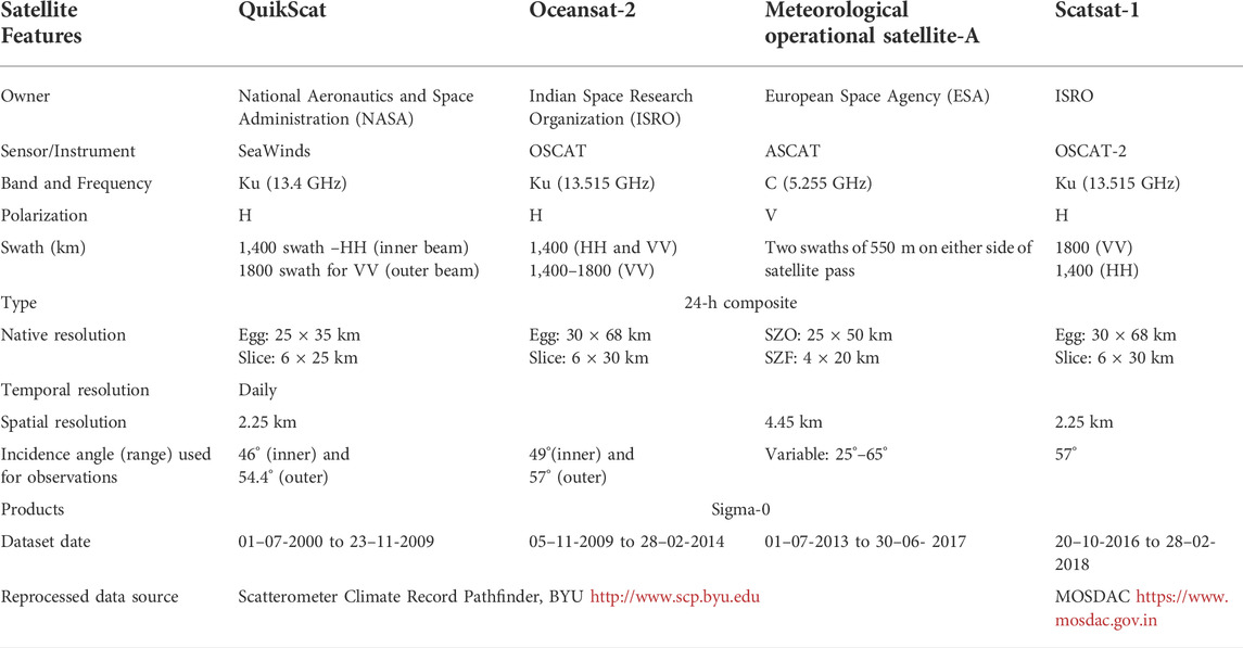
TABLE 1. Data sources and Scatterometer characteristics.

The σ⁰ from QuikSCAT measurements which are used to make slices and eggs are two types. The nominal pixel resolution of egg-based SIR images is 4.45 km, with an estimated effective resolution of 8–10 km, whereas the notional pixel resolution of slice-based SIR images is 2.225 km, with an estimated effective resolution of 5 km. Individual σ⁰ readings have been corrected for incidence angle to the nominal reference angle using a B value of roughly 0.13 dB/deg in a slice-based SIR product.

Since its launch in June 1999, the SeaWinds/QuikSCAT has been operating in dual-polarization mode on the Ku band (13.4 GHz). We employed H-polarized, 2.225 km resolution at an incidence angle of 46° for the period July 2000 to November 2009, processed using the Scatterometer Image Reconstruction (SIR) technique. We used OSCAT/Oceansat-2 H-polarized σ⁰ data with a 48° incidence angle from November 2009 to February 2014. The Indian Space Research Organization (ISRO) launched the Oceansat-2 satellite in September 2009, as a follow-up mission to the QuikSCAT satellite which was turned off in October 2018.

ASCAT/MetOp-A is a dual-fan-beam C-band scatterometer with V-polarization that operates at 5.255 GHz. The σ⁰ is made up of SIR images recorded at 4.45 km with an incidence angle of 48.9°, for the period July 2013 to July 2017. Thereafter, we used 2.25 km resolution OSCAT-2/ScatSat-1 σ⁰ data normalized to a 0° incidence angle for the period October 2016 to February 2018. It was launched by ISRO in October 2016 with specifications similar to Oceansat-2. From November 2000 through February 2018, the σ⁰ time series spans eighteen austral summer melt seasons. To avoid splitting the summer, the melt season runs from 1 November of the previous year to 28 or 29 February of the following year, and is simply referred to as the second year (i.e., summer 2000–01 is just referred to as 2001).

2.1.2 Model reanalysis data

To account for the net heat flux and its possible role in surface melt, we used the heat flux parameters on 0.25° × 0.25° resolution based on the monthly forecast. These data comes from the fifth-generation ECMWF global climate and weather reanalysis (ERA5). The ERA5 atmospheric and land reanalysis has a resolution of 31 km on a Gaussian grid (Tl639) and 63 km for ensemble members (TL319). The vertical component of the atmospheric component consists of 137 levels from the surface to 1 Pa.

2.1.3 Automatic weather station data

Raw data obtained at varied temporal resolutions ranging from 10 min to 3 h were used to create single daily measurements from the NCDC GSOD database. Five AWS were chosen to cover a wide range of melting regimes, with a focus on temporal data continuity and data quality throughout austral summer. These were at 70.89°S, 69.87°E (Emery G3 run by Australia), 72.2°S, 60.16°W (Butler Island operated by UK), 75.86°S, 59.15°W (Limbert operated by UK), 70.66°S, 8.25°E (Neumayer operated by Germany), and 73.2°S, 127.05°W (Emery G3 operated by Australia) (Mount Siple operated by the United States). The air temperature data from these nearby AWS allowed us to establish relationship between surface melt and air temperature (Figures 2, 3).

FIGURE 2

FIGURE 2. A time series of QuikSCAT-based σ0 (blue line) overlaid on daily temperature (red line) at the Amery G3 AWS site (70.8919°S, 69.8725°E). Variable yearly melt thresholds computed using the right-hand side of Eq. 1 for July-September for this site are shown by horizontal green bars. When σ0 drops below the threshold during austral summer, i.e., December- February (magenta boxes), the day is characterized as melting according to Eq 1. The time series begins on 1st July 2000.

FIGURE 3

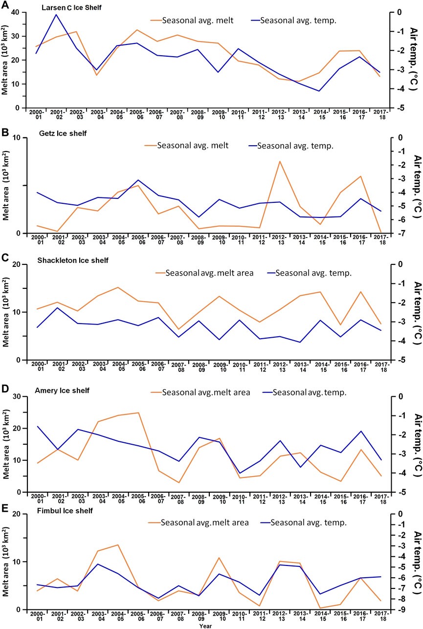
FIGURE 3. Relationship between snow melt-area and air temperature during austral summer for (A) Larsen C ice shelf, (B) Getz ice shelf, (C) Shackleton ice shelf, (D) Amery ice shelf, and (E) Fimbul ice shelf.

2.2 Methodology

2.2.1 Melt detection

The impact of small amounts of liquid water on the electrical properties of snow at microwave frequencies is used to detect melt. Because microwaves penetrate a dry winter snowfall readily, dispersion from the air-snow contact can be ignored (Rott et al., 1996; Kunz and Long, 2006). Volume scattering/ scattering from individual snow grains and inner layers determine the microwave backscatter response in the snowpack (Ulaby et al., 1986). The largest change in electrical properties occurs in the imaginary component of the dielectric constant when merely 0.5% liquid water is introduced through surface melt (Ulaby et al., 1986). The presence of liquid water in the snowpack enhances microwave absorption, decreases penetration depth and subsurface scattering, and reduces σ⁰ (Ashcraft and Long, 2006; Ulaby et al., 1986; Wang et al., 2007). Similarly, σ⁰ may rise during a refreeze, and plummet once snowmelt resumes. Figure 2 shows the variation of the σ⁰ signal vis-à-vis the air temperature (Ta).

While microwave measurements are used to detect the melt, liquid water may be present even when the air temperature is below 0°C, depending on other surface energy balance factors. In this context, the term “melting conditions” refers to either snowmelt or liquid water from a previous melt that is refreezing. Depending on the satellite data used, many researches have suggested alternative strategies for detecting melt. Long (2006) employed the greatest likelihood ratio approach to predict ice-states based on the polarisation ratio, which is the ratio of H-polarization and V-polarization backscatter data. The ratio of probability density functions is calculated using their method (PDF). For the detection of melt/freeze across Antarctica, Bothale et al. (2015) used an adaptive threshold-based classification. This adaptive threshold-based classification approach estimates melt/freeze based on the previous austral winter mean, standard deviation, and drop-in backscatter coefficient for austral summer. Some studies have utilised other ways to detect the melt condition, such as using a predetermined threshold.

We used adaptive threshold-based classification in this investigation, which is similar to that used previously (Ashcraft and Long, 2006; Trusel et al., 2012, Barrand et al., 2013), although with a few tweaks. We found minor fluctuations in backscatter during austral winter after evaluating the time-series of backscatter coefficient. To investigate how this scenario affected the computation, we estimated the mean and standard deviation during the austral summer, and based on mean minus two standard deviations, we calculated the melt detection threshold. When we applied these estimated thresholds to these points, we realized that it had been classified incorrectly because the classification takes into account the transition period under melt. To address this issue, we conducted a transition period study to determine a fluctuation range in that period; this fluctuation was then assessed for all points (Fig. 1), yielding a fluctuation range of 0–2 dB. The criterion was redefined by taking the transition period into account because the value was very high. As a result, we subtracted a fixed value c (Eqs. 1 and 2), and these points revealed significant melt and non-melt days for a given pixel. We define melt on a pixel-by-pixel basis using a σ⁰ threshold approach (e.g., Ashcraft and Long, 2006; Trusel et al., 2012), such that:

$MP=True,if{\sigma }_{dn\le }^0({\sigma }_{wm}^0-3*{\sigma }_{wsd}^0)-c(1)$

$MP=False,if{\sigma }_{dn}^0>\left({\sigma }_{wm}^0-3*{\sigma }_{wsd}^0\right)-c(2)$

In the above equations, MP is melt pixel provide space between pixel and σ⁰ dn ${\sigma }_{dn}^0$ is the backscatter for the nth day and ${\sigma }_{wm}^0$ is the austral winter mean, ${\sigma }_{wsd}^0$is the standard deviation of austral winter period, and c is a constant (=1dB), which is calculated from the transition period for particular pixels. This value is consistent with earlier investigations that employed QuikSCAT data and used empirically calculated constants as follows. Wang et al. (2007) used 2 and 3 dB for Greenland, Wang et al. (2008) used 1.7 dB for pan‐Arctic snowmelt, and Sharp and Wang (2009) used 3.5 dB and 5 dB on Eurasian Arctic ice caps, while Rotschky et al. (2011) used 1.65 dB over Svalbard, and Trusel et al. (2012) used 2 dB for Antarctica. Since our method considers any day below the threshold as melting, it is more sensitive to short-duration melting episodes, when compared to studies designed to detect only incessant melting (e.g., Wang et al., 2007; Tedesco et al., 2007). Other researchers used a simplified equation where melt were determined when σ⁰ was at least 3 dB lower than the winter σ⁰ measurements for C-band (Luckman et al. 2014; Zheng and Zhou, 2020).

What are the consequences of using 1 dB as a constant? Because σ⁰ is dependent on other elements, such as wet snow layer thickness and other inherent snowpack features, it is impossible to set a single threshold for specific snowpack liquid water content (LWC) (Winebrenner et al., 1994; Nghiem et al., 2001; Ulaby et al., 1986). Nagler and Rott (2000) found a 2-dB reduction in σ⁰ for an upper snowpack layer with 1% wetness using C-band (5.3 GHz) measurements, while Ashcraft and Long (2006) modelled the Ku band (13.4 GHz) response to wetness and reported a 3 dB reduction in σ⁰ for a 3.8 cm snow layer with 1% LWC. This value is comparable with experimentally determined dynamic responses to 1.3% LWC, which range from ∼3.5 dB (at 8.6 GHz) to ∼8 dB (at 17 GHz) (Stiles and Ulaby, 1980). Therefore, it can be confidently assumed that a 1 dB threshold using 13.4 GHz QuikSCAT data should represent an upper snowpack of less than ∼1% LWC by volume, thus making our detection scheme highly sensitive. This LWC value compares favorably with PMW melt detection algorithms based on modeled wetness values of 0.2–0.5% (Tedesco et al., 2007), and 0.1–0.2% (Tedesco (2009).

2.2.2 Determining melt-onset dates

Melt-onset (MO) dates are necessary to know the inter-annual variations of surface melt over Antarctic ice shelves. Many studies have been conducted in the past to determine the melt-onset over Arctic and Antarctic sea ice. SAR and scattterometer data were utilised by Winebrenner et al. (1994) to predict the melt beginning of Arctic sea ice. Kunz and Long (2006) employed scatterometer data with the criterion that the first day would be a melt-onset date if the following 3 days were under melt, and that the first day of no melt would be considered a refreezing date if there was no melt for at least 7 days.

For a particular pixel, we regarded five consecutive days to be under melt condition, with the first day being deemed melt-onset day. This approach has been used to determine the melt beginning date for each austral summer month, which is expressed as the actual date for convenient reference. In the summertime σ⁰ time series, the melt duration is measured from the first melt onset date to the last melt onset date.

3 Results

3.1 Mean melt duration

The map of average melt duration over the austral summer from 2000–2018 is portrayed in Figure 4. In Region-A, the Ronne-Filchner Ice shelf experienced an average melt of less than 5 days, while the George VI and Wilkins Ice shelves exhibited the MD >60 days. Likewise, the northern portion of Larsen Ice shelf experienced >60 days, while the southern part exhibitted 35 days of melt. In the Region-B, less spatial variability was observed. Abbott Ice shelf experienced 20–30 days of melt, while Getz and Sulzberger Ice Shelves showed 10 days melt. While the Ross Ice Shelf had a MD of just 5-day, the Shackleton ice shelf, which is located slightly north of the other shelves in Region C, had a relatively long MD of roughly 55 days. Amery and West ice shelves exhibited melt of about 41 days. In Region D, where the MD persisted for around 30 days, Riiser Larsen had the least amount of melt, lasting about 10 days.

FIGURE 4

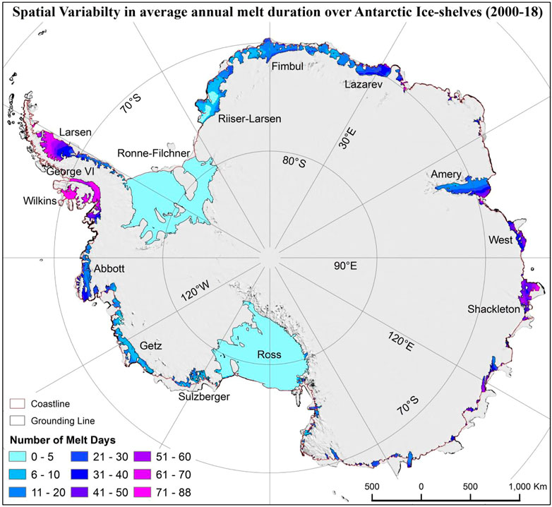
FIGURE 4. Average annual melt duration during austral summers from 2001 to 2018.

3.2 Annual melt onset and melt duration

MD has important implications on the health of the ice sheet. Longer melt duration leads to the formation of melt ponds on sea ice and ice sheets, which in turn absorb more solar radiation and induce further snowmelt through melt-albedo feedback (Bell et al., 2018). The timing and extent of surface snowmelt are indicators of changes in polar climate and thus and thus potentially have regional and global climate implications. Figures 5 and 6 show maps of MO date and spatial-average time series for different shelf locations, whereas Figures 7 and 8 show maps of MD and spatial-average time series throughout the austral summer. The maps demonstrate the expansion/contraction of snow melt in space and time illustrate that snow melt increases and decreases in space and time. The MO was on 330 ± 12 (25 November, on average) and the mean MD was 60 ± 14 days across the shelves in Region A. The shelves in this region exhibited an early MO and highest MD. Among the three shelves, the Wilkins Ice shelf experienced earliest MO on 324 ± 13 (19 November), and a longest MD of 80 ± 16 days. This was followed by George Ice shelf with a MO on 331 ± 16 (25 November), with MD of 61 ± 18 days. The Larsen Ice shelf showed a MO on 336 ± 16 (1 December), with MD of 40 ± 26 days. However, Filchner-Ronne Ice shelf experienced melt only during 2001–02, 2002–03, 2006–07, 2007–08, 2008–09, 2014–15.

FIGURE 5

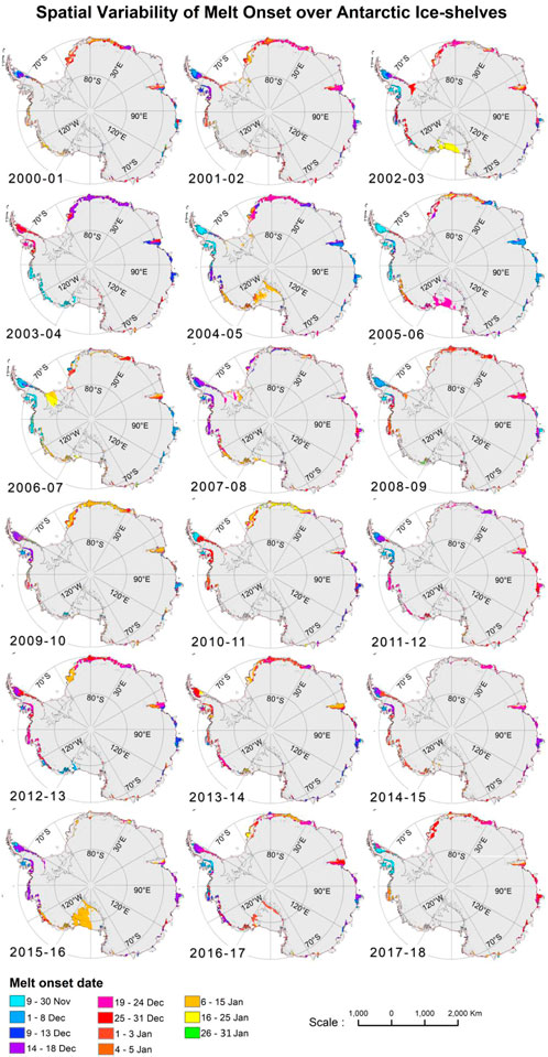
FIGURE 5. Spatial extent of melt onset during austral summer from 2001 to 2018.

FIGURE 6

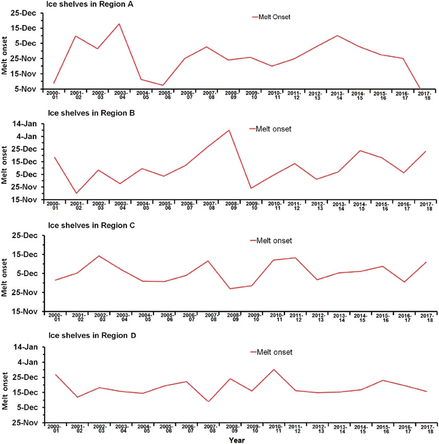
FIGURE 6. Time series of spatial-averaged melt onset at different regions demarcated in Figure 1.

FIGURE 7

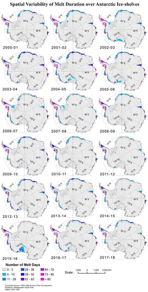
FIGURE 7. Melt duration in Antarctica during austral summer from 2001 to 2018.

FIGURE 8

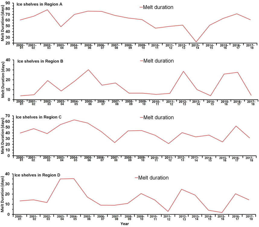
FIGURE 8. Time series of spatial-averaged melt duration at different regions demarcated in Figure 1.

The AP’s shelves have the highest amount of melt days, with an annual average MD of about 70 days. For over half of the region, MO was detected fairly early, around November 20. Early MO began across the entire region in the first or second week of November in the years 2004–05, 2005–06, and 2006–07. The MD and MO findings are in line with other studies carried out by other researchers during the specified time period. For example, a decreasing trend in MD of one day/year for AP is consistent with that reported elsewhere (Bevan et al., 2018). The average MD and MO indicated in this study are consistent with Wang et al. (2018).

The Larsen-C Ice shelf recorded higher melting rates as compared to the other ice-shelf. The entire Larsen-C shelf experienced melt for maximum of 70 days and half of the shelf’s area experienced melt for more than 90 days. This shelf recorded decreasing melt duration austral summer from 2001–02 to austral summer of 2010–11 and after that no significant trend was seen; the duration of the melt during 2010–11 to 2017–18 experienced fluctuation that showed less number of melt days as compared to the period 2000-01 to 2009–10. MO on the Larsen-C Ice Shelf began in November of the first decade (2000–2009). The lone austral summer in the first decade, 2003-04, saw melting begin around the end of December/first week of January. There was no discernible trend in MO during the following decade (2009–2017). MO at ice shelf was seen in the first week of November during 2017–18. More than 40,000 square km area of Larsen-C ice shelf or entire area of the shelf experienced melt continuously for than 60 days for the years 2005, 2006, and 2007 which started in the first week of December and ended with decreasing melt area to the end of the February or therafter. The shelf shows significant decrease in melt area as compared to first decade of this study. It was observed that 19–24% of the ice shelf area of the Larsen-C experienced melt from 2000–01 to 2002–03, and from 2004–05 to 2009–10, while in 2003–04 and from 2010–11 to 2017–18, 10–18% of the shelf area melted. In summary, along the Larsen-C ice shelf, a shifting pattern in melt onset was observed.

In Region B, MO occurred on 346 ± 12 (11 December) on the shelves, with an average MD of 13 ± 9 days. The average MO (MD) for Abbott Ice Shelf was 340 ± 17 (23 ± 17 days), 346 ± 18 (9 ± 8 days), and 352 ± 45 (9 ± 8 days) for Getz and Sulzberger Ice Shelves, respectively. Getz Ice Shelf is one of the shelves in the west Antarctic region that has experienced the least melting. Getz Ice Shelf is one of the shelves in the west Antarctic region that has experienced the least melting. We found increased melt in austral summer of 2005–06, 2012–13, 2015–16, and 2016–17, which lasted about 15–20 days, which was relatively low in comparison to other large ice shelf.

Getz Ice-shelf also experienced the least amount of melt in the west Antarctic region, where many of the shelves melt rapidly during austral summer (Rignot et al. 2013, Paolo, et al. 2015). During austral summers of 2005–06, 2012–13, 2015–16, and 2016–17, the ice shelf experienced increased melt in the first and second weeks of January, which was about 15–20 days, which is very low as compared to other major ice shelves under study. Several austral seasons, there was no or very little melt across the shelf, or the melt was very brief (<15 days).

The typical pattern of MO was the first/second week of January across the whole Getz Ice Shelf area. During the summers of 2008–09, 2009–10, and 2010–11, very little shelf area (on average < 1,200 km² per day) was under melt. During the austral summers of 2005–06, 2012–13, 2015–16, and 2016–17, the entire shelf, which covers more than 30,000 km², witnessed melt for just 9, 12, 7, 13 days, respectively.

The average MO for Region C was 341 ± 5 (6 December), with MD of 41 ± 12 days. It is noted that the MO for Shackleton Ice Shelf, the southernmost shelf, was 334 ± 10 (19 November), lasting a duration of 50 ± 14 days on average. On the other hand, the MO/MD for the West Ice Shelf was found to be 340 ± 8 (5 December)/39 ± 14 days on average; while the MO for the Amery Ice Shelf was 347 ± 10 (12 December)/32 ± 18 days on average.

MD on the Shackleton Ice Shelf has been increasing. The number of melt days has grown during the last 2 decades (2000–09, 2009–2017). During the austral summers of 2013–14 and 2016–17, the longest melt period of more than 80 days was observed. The shortest melt duration was seen during the austral summer of 2015–16, when the AP saw a period of high melt. The average MD in the eastern Antarctic region was roughly 60 days, which is extremely long. In the eastern Antarctic region, the typical MD was about 60 days, which is a very lengthy time. East Antarctica’s Shackleton Ice Shelf demonstrated unusually early melt beginning in the first or second week of December, 15 days earlier than the AP region.

The Shackleton Ice Shelf, which has a high geographic coverage of more than 30,000 km², is the second Ice Shelf to melt between 2004 and 2017, following the Larsen-C Ice Shelf, with an ice shelf size of roughly 33,800 km². The MO was found to be 353 ± 5 (18 December) for shelves in the northern part of Antarctica (Region D), with an average MD of 15 ± 9 days. The MO for all three ice shelves was 16–20 December, with the MD spanning from 12 to 22 days for the Riiser-Larsen Ice Shelf and the Lazarev Ice shelf.

Fimbul Ice Shelf had the longest melt during 2003–2005, with an average of about 40 days. The MO for this shelf was typically mid-December, but in 2009–10 and 2010–11, it was in January. No melt was identified the following year, and the MO changed back to mid-December. No melt was found the following year, and the MO changed back to mid-December. With an average melt area of less than 1300 km2 each day from the start of the melt to the finish, the MD for 2014–15 was incredibly brief. The largest melt area during the austral summer of 2004–2005 was 40,000 km², and it lasted for more than 30 days.

In conclusion, the ice shelves in Region A experienced MO from 10 November to 15 December together with a lengthy MD (>50 days) between 2000 and 2013. In Region B, the MD ranged from 20 to 60 days, while the MO was approximately 15 December. The melt duration was 35 days on the ice shelves in the other two locations.

3.3 Snow melt area

The area under melt and the MO day for Larsen C, Amery, Getz, Shackleton and Fimbul Ice Shelves are shown in Figure 9. The horizontal line represents a 95% confidence level. Between 13 December and 12 February, the Larsen Ice Shelf showed a considerable increase in melt area. The Amery and Shackleton ice shelves experienced increased and significant melting from 16 December to 2 February and 10 December to 7 February, respectively. The melt area on the Fimbul and Getz ice shelves dramatically increased over the weeks of 18 December to 31 January and 23 December to 24 January, respectively. It is noted that for Amery, Getz, Shackleton, Larsen, and Fimbul, the temporal variation of melt area showed a decreasing trend of 196 km²/yr, which is significant at 95% confidence interval.

FIGURE 9

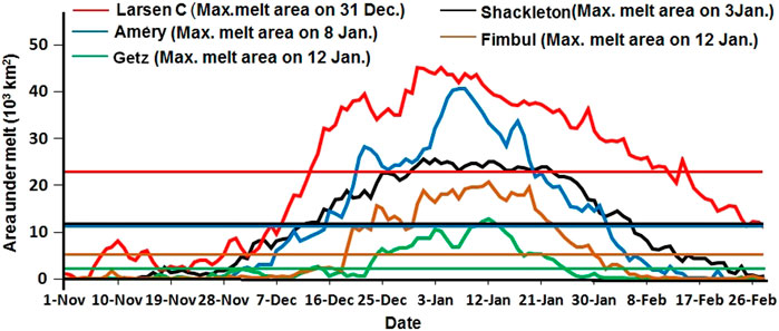
FIGURE 9. Melt area versus the onset day for selected ice shelves. Horizontal lines indicate 95% confidence level.

Of the total ice shelf area of 70,000 km², Larsen C Ice Shelf experienced an average melt of 22,685 km² over the 2000–2018 period. More than 35% of the ice shelf experienced melt during 2000 to 2003, and 2004 to 2010. For the Getz Ice Shelf, we found that >10% of melt area occurred during 2004 to 2006, and the highest melt area of 23% were detected during 2012–13. The average melt area was found to be 2471 km² out of the total shelf area of 32,790 km². For the Shackleton Ice Shelf, with a total of 29,870 km², the average melt area over the entire period of analysis was found to be 11,200 km². We detected >40% melt area during 2001–02, 2003 to 2007, 2009–10, 2013 to 2015, and 2016–17. As for Amery Ice Shelf, whose total area amounts to 60,800 km² the average melt area over the period of analysis was found to be 11,406 km². We detected melt area >35% of the total shelf area during 2003 to 2006. On the other hand, the Fimbul Ice Shelf, with a total area of 60,660 km², experienced the least melt area which on average was 5500 km² for the period 2000–2018, and the melt area >20% was found during 2003 to 2005.

Figure 10A shows the time series of annual surface melt area and the trends for a few ice shelves. The trend in the melt area over the 18-year period showed a highest decreasing trend of −79.8 km²/yr (p < 0.05) which translates into 15% surface melt variability (between 2000–01 and 2017–18) for Larsen-C Ice Shelf. On the other hand, the lowest decreasing tendency of −14.3 km²/yr (not significant) and 10% surface melt variability (between 2000–01 and 2017–18) was detected for Shackleton Ice Shelf. Amery Ice Shelf exhibited. After Larsen C, the surface melt on the Amery Ice Shelf showed a decreasing trend of −76.7 km²/yr (significant at 95% confidence interval) and 46% surface melt variability (between 2000–01 and 2017–18). The decreasing surface melt trend for Fimbul Ice Shelf of −29.9 km²/yr (not significant) and surface melt variability of 56% between 2000–01 and 2017–18. It is noted that the Getz Ice Shelf exhibited a positive melt trend of 4.2 km²/yr (not significant) and a surface melt variability of 66% between 2000–01 and 2017–18. The trend for the total surface melt area for all these shelves showed between 2000–01 and 2017–18 (Figure 10B).

FIGURE 10

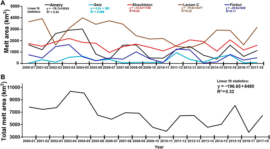
FIGURE 10. (A) Surface melt-area time series for a selected ice shelves. (B) total area under melt for all the ice shelves in panel 9A.

3.4 Relationship between air temperature and snow melt area

During the austral summer, snow melt is triggered by surface warming due to solar radiation. We chose a few ice shelves to represent the four sectors illustrated in Figure 1 based on the availability of weather data. For the Larsen C Ice Shelf, a substantial and significant connection (R = 0.71, p < 0.01) was discovered between melt area and average austral air temperature (Figure 10A). The Getz Ice Shelf experienced a significant interannual variability, according to a modest but not statistically significant correlation between the two measurements (Figure 9). For the Shackleton Ice Shelf, we discovered a significant correlation (R = 0.40, p < 0.05) between austral mean temperature and melt area (Figure 10C). Similarly, for the Amery and Fimbul Ice shelves, the respective correlation between air temperature and melt area was 0.46 (p < 0.05) and 0.81 (p < 0.01), indicating the important of the former (Figures 10D,E). The topographic impacts are reflected in the weaker linear correlation between melt extent and air temperature. Due to the comparatively steep slope of the continental ice sheet’s coastal zone, melting further inland would proceed at a slower rate than predicted by linear regression models as sea temperatures rose (Liu et al., 2006).

4 Discussion

Melt extent, MO date, and MD were derived using scatterometer-based σ⁰ data from 2000 to 2018, using the pixel-based adaptive threshold approach, with the constant value generated by examining change in σ⁰ throughout the transition period between winter and summer.

MD over Antarctica’s ice shelves has revealed a distinct spatial distribution pattern according on its position on the continent. The shelves on the AP showed a pattern of increasing melt from the northwestern region of the shelf to the south; the Amery Ice-Shelf in the eastern region of Antarctica showed a pattern of high melt over the north-eastern region with less MD and melt extent over the western ice-shelf region.

Parts of the Wilkins, Larsen C, and George IV Ice Shelves, as well as western AP outlet glaciers, showed an average MD of 70 days per year on the AP, while Trusel et al. (2012) used passive microwave data and a wavelet transform-based method detected MD of over 100 days. The MD and extent are critical for understanding Larsen-C’s stability. For example, researchers have identified Larsen C Ice Shelf as being vulnerable to hydrofracturing-mediated collapse as the climate warms (Trusel et al., 2015; Lai et al., 2020).

The Fimbul Ice Shelf, which is centred on 0° and located at the perimeter of the Antarctic ice sheet, exhibitted a completely different pattern of melt extent and MD, indicating that other factors, in addition to coastal location, contribute to surface melting over this region. Our results suggest that Fimbull Ice Shelf exhibited least melt area which on average was 5500 km² for the period 2000–2018, and the melt area was below 18% for the analysis period, except for 2003 to 2005.

MO over the Antarctic ice shelves showed a considerable shift in the date over the period 2000–2018 on some shelves, but no significant changes on other shelves. During the first decade of this study, most of the ice-shelves on the Larsen-C revealed a considerable change in the melt onset date to the first/second week of December, which was previously observed in the first/second week of November.

Melting occured over the ice shelves of the AP and the west Antarctic region as a result of atmospheric wind circulation. The western coast of AP experiences higher melt duration due to higher solar radiation intensity at lower latitudes and advection of warm humid air masses from northerly directions, as opposed to the eastern coast, which gets cooler winds from Antarctica’s inland region. Scambos et al. (2000) hypothesised that the collapse of ice shelves on the Antarctic Peninsula (Vaughan and Doake, 1996; MacAyeal et al., 2003) was linked to ponded water produced by lengthy and extensive ice shelf melt. Even though the sea surrounding the shelf sees increased heat in the austral summer, wind direction and air circulation could be one of the Ross Ice Shelf melting slowly or not at all in some years.

The shelves on the Queen Maud Land region, the Amery Ice Shelf region, and the Shackleton Ice Shelf all melted steadily and extensively, whereas the shelves on Wilkes Land and Marie Byrd Land melted quickly along a narrow coastal band. The Ronne-Filchner Ice Shelf and the Ross Ice Shelf had the lowest melt duration (no melt was observed in some years) and the greatest interannual fluctuation in melt area, according to our findings. According to our melt analyses, melt area trend on the West Ice Shelf, Shackleton Ice Shelf, and Amery Ice Shelf was found to be −60, −84, −548 km²/yr as well as the ice shelves along the Princess Ragnhild Coast in Queen Maud Land (Fimbul Ice Shelf: −202 km²/yr), was likewise quite continuous and intense during the study period. These ice shelves may be vulnerable to breakup if surface melting intensifies further, thus they should be continuously monitored. The preview of this work does not go into the causes of MD, MO, or melt extent, although it is noted that the atmospheric circulation affects the melting scenario.

The air pressure in the Indian Ocean is unusually low in the eastern part of Antarctica, near the Shackleton Ice Shelf, during the austral summer of each year, compared to the interior region of Antarctica. The heat flow gradient towards the Shackleton Ice Shelf is very significant, ranging from roughly 60 W/m² to 120 W/m² over a short distance (Supplementary Figure 1A). This makes the area amenable to fluctuations in surface temperature caused by wind circulation, which is one of the elements affecting and modulating surface temperature over east Antarctica’s ice shelves.

The extent of melt on some Antarctic ice shelves is also influenced by air temperature advection. We found a distinct pattern of increased temperature advection from the west of AP and increased melt area across the Amery, Shackleton, and Larsen-C Ice Shelves (Supplementary Figure 1B), although temperature advection during the austral summer over the Fimbul Ice shelf was not the cause for melt extent. The temperature advection on the Getz Ice shelf was reduced due to the wind direction (Supplementary Figures 1A,B), which emerged from the interior of Antarctica toward the coast and carried a comparatively cooler air mass, lowering the temperature over the shelf which resulted in less melt area/less MD.

Literature emphasises the importance of the Southern Annular Mode (SAM) and the Southern Oscillation Index on Antarctic surface melt (SOI). Strong SAM and SOI dominate the high southern latitude air circulation, and poleward heat propagation is conducive to surface melt, according to some research (Torinesi et al., 2003; Tedesco and Monaghan, 2009). During the 1979–2009 period, Tedesco and Monaghan (2009) discovered that negative melt index and extent are highly linked with the combined positive anomalies of SAM and SOI. In our analysis, the combined anomalies of SAM and SOI were significantly but negatively correlated with melt area for Shackleton Ice Shelf (R = −0.62, p < 0.05), Amery Ice Shelf (R = −0.54, p < 0.05), and Fimbul Ice shelve (R = −0.49, p < 0.05). Melt was enhanced in the western Antarctic shelves during negative SOI anomalies.

Table 2 shows a comparison of maximum melt day between our results and those of Bothale et al. (2015) using scatterometer data from 2001 to 2014. Our study reveals that the peak melt date for the Amery, Fimbul, and Getz Ice shelves has delayed by a month. The maximum melt area for Larsen-C Ice Shelf was also delayed by around 15 days, and the Shackleton Ice shelf was delayed by 23 days. The very high melt during 2004-05 and low melt during 2007-08 for Amery Ice Shelf concurs with the results portrayed in Oza (2015) who used QuikSCAT and OSCAT backscatter data to investigate the spatially varying pattern of melt from 2000 to 2010. They reported low intensity surface melting (<3 dB per summer) over the large Filchner-Ronne and Ross ice shelves and almost 40 times higher on AP for the period 2000–2010, which agrees with inference drawn in this study.

TABLE 2

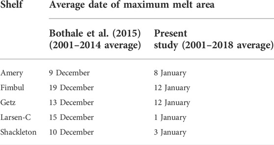
TABLE 2. Comparison of maximum surface snow melt area with the earlier study done on Antarctic ice shelves.

One of the significant findings from our analysis was that the total melt area over the ice shelves shows a decreasing trend of 196 km²/yr (statistically significant at 95% and 97% confidence interval) over the 18-year period. However, it is recommended that analysis is extended for further period to draw a definitive conclusion. The melting of ice shelves on Antarctica is crucial because it is sensitive to changes in air and ocean circulation around the continent. The melting of ice shelves on Antarctica is crucial because it is sensitive to changes in air and ocean circulation around the continent. The flow of glaciers speeds up as an ice shelf collapses, making the ice sheet vulnerable to disintegration. Because the melt and freeze condition is extremely dynamic and has considerable interannual fluctuation, it must be monitored on a regular basis. Furthermore, quantitative data on snowmelt extent and duration will be essential input for climate and sea level change modelling and prediction.

5 Conclusion

Using a time series of radar backscatter data from QuikSCAT, OSCAT, ASCAT, and OSCAT-2, surface melting dynamics over the Antarctica ice shelves have been addressed. We provided maps of MO and MD, and time series of melt index. MD and MO do not always change linearly over distance and time, particularly in areas where increased melting occurs over the AP’s Ice Shelves. The Ronne-Filchner and Ross Ice Shelves melted in less than 5 days on average, whereas the George VI, Wilkins, and northern portion of the Larsen Ice Shelf melted in more than 60 days. Abbott Ice shelf experienced 20–30 days of melt in the west Antarctic, while Getz and Sulzberger Ice Shelves exhibited 10 days melt. On average, the Shackleton, Amery and West Ice shelves had a MD of 40–55 days. The least spatial variation was seen in northern Antarctica, where the melt lasted 30 days, with RiiserLarsen Ice Shelf having the shortest melt of 10 days.

For over half of the region on the AP, the melt onset was November 20. MO the Larsen-C Ice Shelf began on 25 November. After Larsen-C Ice Shelf, Shackleton Ice Shelf is the second ice shelf where melt occurred during 2004–05 and 2016–17 with high spatial coverage of more than 30,000 km². MO dates for ice shelves in the northern Antarctic ranged from 16 to 20 December, with MD ranging from 12 to 22 days for the Riiser-Larsen Ice Shelf and the Lazarev Ice Shelf. Melt began on shelves in the southwest Antarctic region on December 15 and continued for 20–60 days. The MO for Amery and West Ice Shelves was between 1 and 15 December.

For the Larsen, Shackleton, Amery, and Fimbul Ice shelves, there was a substantial link between melt area and average austral air temperature. There was a clear pattern between increased temperature advection and increased melt area for Amery, Shackleton and Larsen-C Ice Shelves. The teleconnections found between melt area and the combined anomalies of SAM and SOI point to the high southern latitudes being coupled to the global climate system. Similarly, significant melting events on the Ross Ice Shelf and on West Antarctica appear to be exacerbated by low SOI. These time-series measurements add to our understanding of the spatiotemporal dynamics of surface melting in the Antarctic, a process that is particularly crucial to monitor when gauging the stability of Antarctic ice shelves in the context of sustained atmospheric warming.

Data availability statement

The original contributions presented in the study are included in the article/Supplementary Material, further inquiries can be directed to the corresponding author.

Author contributions

AL conceptualized the problem and wrote the paper, MA processed the data under the supervision of SJ.

Acknowledgments

We thank NCPOR Director M. Ravichandran for faculties to carry out this work. Authors acknowledge the use of AWS data which was downloaded from https://amrc.ssec.wisc.edu/. ERA5 heat flux and meteorological data were downloaded from https://cds.climate. Copernicus. eu/. The SAM index was obtained from https://climatedataguide.ucar.edu/climate-data/marshall-southern-annular-mode-sam-index-station-based, while SOI was downloaded from https://www.ncdc.noaa.gov. This is NCPOR contribution No J-30/2022-23.

Conflict of interest

The analysis addressed in this work was carried when AM was an internship. student at the National Centre for Polar and Ocean Research, MoES, India. Thereafter, AM sought an employment at the RMSI Private Limited, India.

The remaining authors declare that the research was conducted in the absence of any commercial or financial relationships that could be construed as a potential conflict of interest.

Publisher’s note

All claims expressed in this article are solely those of the authors and do not necessarily represent those of their affiliated organizations, or those of the publisher, the editors and the reviewers. Any product that may be evaluated in this article, or claim that may be made by its manufacturer, is not guaranteed or endorsed by the publisher.

Supplementary material

The Supplementary Material for this article can be found online at: https://www.frontiersin.org/articles/10.3389/frsen.2022.953733/full#supplementary-material

SUPPLEMENTARY FIGURE S1 | (A) Distribution of mean net heat flux, wind speed, and sea level pressure during astral summer; and (B) temperature advection across the Antarctic shelves.

References

Abdalati, W., and Steffen, K. (2001). Greenland ice sheet melt extent: 1979–1999. J. Geophys. Res. 106 (D24), 33983983989–33984033988. doi:10.1029/2001jd900181

CrossRef Full Text | Google Scholar

Abdalati, W., and Steffen, K. (1995). Passive microwave‐derived snow melt regions on the Greenland ice sheet. Geophys. Res. Lett. 22 (7), 787–790. doi:10.1029/95gl00433

CrossRef Full Text | Google Scholar

Abdalati, W., and Steffen, K. (1997). Snowmelt on the Greenland ice sheet as derived from passive microwave satellite data. J. Clim. 10, 3165–3175. doi:10.1175/1520-0442(1997)010<0165:sotgis>2.0.co;2

CrossRef Full Text | Google Scholar

Anderson, M. R. (1987). The Onset of Spring melt in first-year Ice Regions of the Arctic as determined from Scanning Multichannel Microwave Radiometer data for 1979 and 1980, Papers in the Earth and Atmospheric Sciences, 182. Available at: https://digitalcommons.unl.edu/geosciencefacpub/182.

CrossRef Full Text | Google Scholar

Armstrong, R. L., Knowles, K. W., Brodzik, M. J., and Hardman, M. A. (2003). DMSP SSM/I pathfinder daily EASE‐grid brightness temperatures. Boulder, Colo: Natl. Snow and Ice Data Cent. Available at: http://nsidc.org/data/docs/daac/nsidc0032_ssmi_ease_tbs.gd.html

Google Scholar

Ashcraft, I. S., and Long, D. G. (2006). Comparison of methods for melt detection over Greenland using active and passive microwave measurements. Int. J. Remote Sens. 27, 2469–2488. doi:10.1080/01431160500534465

CrossRef Full Text | Google Scholar

Banwell, A. F., MacAyeal, D. R., and Sergienko, O. V. (2013). Breakup of the Larsen B Ice Shelf triggered by chain reaction drainage of supraglacial lakes. Geophys. Res. Lett. 40, 5872–5876. doi:10.1002/2013GL057694

CrossRef Full Text | Google Scholar

Banwell, A. F., Willis, I. C., Macdonald, G. J., Goodsell, B., and MacAyeal, D. R. (2019). Widespread movement of meltwater onto and across Antarctic ice shelves. Nature 544, 349510–350352. doi:10.1038/nature22049

CrossRef Full Text | Google Scholar

Banwell, A. F., Datta, R. T., Dell, R. L., Moussavi, M., Brucker, L., and Picard, G. (2001). The 32-year record-high surface melt in 2019/2020 on the northern George VI Ice Shelf, Antarctic Peninsula. The Cryosphere 15, 909–925. doi:10.5194/tc-15-909-2021

CrossRef Full Text | Google Scholar

Barrand, N. E., Vaughan, D. G., Steiner, N., Tedesco, M., Kuipers Munneke, P., van den Broeke, M. R., et al. (2013). Trends in Antarctic Peninsula surface melting conditions from observations and regional climate modeling. J. Geophys. Res. Earth Surf. 118 (1), 315–330. doi:10.1029/2012JF002559

CrossRef Full Text | Google Scholar

Bassis, J. N., and Walker, C. C. (2012). Upper and lower limits on the stability of calving glaciers from the yield strength envelope of ice. Proc. R. Soc. A 468, 913–931. doi:10.1098/rspa.2011.0422

CrossRef Full Text | Google Scholar

Bell, R. E., Banwell, A. F., Trusel, L. D., and Kingslake, J. (2018). Antarctic surface hydrology and impacts on ice-sheet mass balance. Nat. Clim. Chang. 8, 1044–1052. doi:10.1038/s41558-018-0326-3

CrossRef Full Text | Google Scholar

Bentley, M. J., Hodgson, D. A., Sugden, D. E., Roberts, S. J., Smith, J. A., Leng, M. J., et al. (2005). Early holocene retreat of the george VI ice shelf, antarctic peninsula. Geol. 33, 173–176. doi:10.1130/g21203.1

CrossRef Full Text | Google Scholar

Bevan, S. L., Luckman, A. J., Kuipers Munneke, P., Hubbard, B., Kulessa, B., and Ashmore, D. W. (2018). Decline in surface melt duration on Larsen C Ice Shelf revealed by the advanced scatterometer (ASCAT). Earth and Space Sci. 5, 578–591.

CrossRef Full Text | Google Scholar

Borstad, C. P., Rignot, E., Mouginot, J., and Schodlok, M. P. (2013). Creep deformation and buttressing capacity of damaged ice shelves: Theory and application to larsen C ice shelf. Cryosphere 7, 1931–1947. doi:10.5194/tc-7-1931-2013

CrossRef Full Text | Google Scholar

Bothale, R. V., Rao, P. V. N., Dutt, C. B. S., Dadhwal, V. K., and Maurya, D. (2015). Spatio-temporal dynamics of surface melting over Antarctica using OSCAT and QuikSCAT scatterometer data (2001–2014). Curr. Sci. 109, 733.

Google Scholar

Campbell, W. J., Gloersen, P., and Zwally, H. J. (1984). “Aspects of Arctic sea ice observable by sequential passive microwave observations from the Nimbus-5 satellite,” in Arctic technology and policy. Editors I. Dyer, and C. Chryssotomidis (New York: Hemisphere), 197–222.

Google Scholar

Cook, A., and Vaughan, D. (2010). Overview of areal changes of the ice shelves on the Antarctic Peninsula over the past 50 years. Cryosphere 4, 77–98. doi:10.5194/tc-4-77-2010

CrossRef Full Text | Google Scholar

DeConto, R. M., and Pollard, D. (2016). Contribution of Antarctica to past and future sea-level rise. Nature 531, 591–597. doi:10.1038/nature17145

PubMed Abstract | CrossRef Full Text | Google Scholar

De Rydt, J., Gudmundsson, G. H., Rott, H., and Bamber, J. L. (2015). Modeling the instantaneous response of glaciers after the collapse of the Larsen B Ice Shelf. Geophys. Res. Lett. 42, 5355–5363. doi:10.1002/2015gl064355

CrossRef Full Text | Google Scholar

Doake, C. S. M., Corr, H. F. J., Rott, H., Skvarça, P., and Young, N. W. (1998). Breakup and conditions for stability of the northern larsen ice shelf, Antarctica. Nature 391, 778–780. doi:10.1038/35832

CrossRef Full Text | Google Scholar

Doake, C. S. M., and Vaughan, D. G. (1991). Rapid disintegration of the Wordie Ice Shelf in response to atmospheric warming. Nature 350, 328–330. doi:10.1038/350328a0

CrossRef Full Text | Google Scholar

Dunmire, D., Lenaerts, J. T. M., Banwell, A. F., Wever, N., Shragge, J., Lhermitte, S., et al. (2020). Observations of buried lake drainage on the antarctic ice sheet. Geophys. Res. Lett. 47, e2020GL087970. doi:10.1029/2020GL087970

PubMed Abstract | CrossRef Full Text | Google Scholar

Early, D. S., and Long, D. G. (2001). Image reconstruction and enhanced resolution imaging from irregular samples. IEEE Trans. Geosci. Remote Sens. 39 (2), 291–302. doi:10.1109/36.905237

CrossRef Full Text | Google Scholar

Fahnestock, M. A., Abdalati, W., and Shuman, C. A. (2002). Long melt seasons on ice shelves of the Antarctic Peninsula: An analysis using satellite-based microwave emission measurements. Ann. Glaciol. 34, 127–133. doi:10.3189/172756402781817798

CrossRef Full Text | Google Scholar

Gardner, A. S., Moholdt, G., Scambos, T., Fahnstock, M., Ligtenberg, S., van den Broeke, M., et al. (2018). Increased West Antarctic and unchanged East Antarctic ice discharge over the last 7 years. Cryosphere 12 (2), 521–547. doi:10.5194/tc‐12‐521‐2018

CrossRef Full Text | Google Scholar

Garrity, K. (1992). “Characterization of snow on floating ice and case studies of brightness temperature change during the onset of melt,” in Ïn Microwave remote sensing of sea ice. Editor F. D. Carsey (Washington, D.C. AGU)

Google Scholar

Glasser, N. F., Scambos, T. A., Bohlander, J., Truffer, M., Pettit, E. C., and Davies, B. J. (2011). From ice-shelf tributary to tidewater glacier: Continued rapid recession, acceleration and thinning of röhss glacier following the 1995 collapse of the prince gustav ice shelf, antarctic peninsula. J. Glaciol. 57 (203), 397–406. doi:10.3189/002214311796905578

CrossRef Full Text | Google Scholar

Glasser, N. F., and Scambos, T. A. (2008). A structural glaciological analysis of the 2002 Larsen B ice-shelf collapse. J. Glaciol. 54, 3–16. doi:10.3189/002214308784409017

CrossRef Full Text | Google Scholar

Holland, P., Corr, H., Pritchard, H., Vaughan, D., Arthern, R., Jenkins, A., et al. (2011). The air content of Larsen ice shelf. Geophys. Res. Lett. 38, L10503. doi:10.1029/2011GL047245

CrossRef Full Text | Google Scholar

Hubbard, B., Luckman, A., Ashmore, D., Bevan, S., Kulessa, B., Kuipers Munneke, P., et al. (2016). Massive subsurface ice formed by refreezing of ice-shelf melt ponds. Nat. Commun. 7, 11897. doi:10.1038/ncomms11897

PubMed Abstract | CrossRef Full Text | Google Scholar

Joshi, M., Merry, C. J., Jezek, K. C., and Bolzan, J. F. (2001). An edge detection technique to estimate melt duration, season and melt extent on the greenland ice sheet using passive microwave data. Geophys. Res. Lett. 28 (18), 3497–3500. doi:10.1029/2000gl012503

CrossRef Full Text | Google Scholar

Kingslake, J., Ely, J. C., Das, I., and Bell, R. E. (2017). Widespread movement of meltwater onto and across Antarctic ice shelves. Nature 544 (7650), 349–352. doi:10.1038/nature22049

PubMed Abstract | CrossRef Full Text | Google Scholar

Kuipers Munneke, P., Ligtenberg, S. R. M., Van Den Broeke, M. R., and Vaughan, D. G. (2014). Firn air depletion as a precursor of Antarctic ice-shelf collapse. J. Glaciol. 60 (220), 205–214. doi:10.3189/2014JoG13J183

CrossRef Full Text | Google Scholar

Kuipers Munneke, P., Luckman, A. J., Bevan, S. L., Smeets, C. J. P. P., Gilbert, E., van den Broeke, M. R., et al. (2018). Intense winter surface melt on an Antarctic ice shelf. Geophys. Res. Lett. 45. doi:10.1029/2018GL077899

CrossRef Full Text | Google Scholar

Kunz, L. B., and Long, D. G. (2006). Melt detection in Antarctic ice shelves using scatterometers and microwave radiometers. IEEE Trans. Geosci. Rem. Sens. 44 (9), 2461–2468.

CrossRef Full Text | Google Scholar

Lai, C.-Y., Kingslake, J., Wearing, M. G., Cameron Chen, P.-H., Gentine, P., Li, H., et al. (2020). Vulnerability of Antarctica’s ice shelves to meltwater-driven fracture. Nature 584 (7822), 574–578. doi:10.1038/s41586-020-2627-8

PubMed Abstract | CrossRef Full Text | Google Scholar

Lhermitte, S., Sun, S., Shuman, C., Wouters, B., Pattyn, F., Wuite, J., et al. (2020). Damage accelerates ice shelf instability and mass loss in Amundsen Sea Embayment. Proc. Natl. Acad. Sci. U. S. A. 117, 24735–24741. doi:10.1073/pnas.1912890117

PubMed Abstract | CrossRef Full Text | Google Scholar

Li, X., Zhang, Y., and Liang, L. (2017). Snowmelt detection on the Greenland ice sheet using microwave scatterometer measurements. Int. J. Remote Sens. 38, 796–807. doi:10.1080/01431161.2016.1271479

CrossRef Full Text | Google Scholar

Liang, D., Guo, H., Zhang, L., Cheng, Y., Zhu, Q., and Liu, X. (2021). Time-series snowmelt detection over the Antarctic using Sentinel-1 SAR images on Google Earth Engine. Rem. Sens. Environ. 256, 112318.

CrossRef Full Text | Google Scholar

Liu, H., Wang, L., and Jezek, K. C. (2006). Spatiotemporal variations of snowmelt in Antarctica derived from satellite scanning multichannel microwave radiometer and Special Sensor Microwave Imager data (1978–2004). J. Geophys. Res. 111 (F1), F01003. doi:10.1029/2005JF000318

CrossRef Full Text | Google Scholar

Long, D, G. (2017). Comparison of Sea winds backscatter imaging algorithms. IEEE J. Sel. Top. Appl. Earth Obs. Remote Sens. 10 (5), 2214–2231. doi:10.1109/JSTARS.2016.2626966

PubMed Abstract | CrossRef Full Text | Google Scholar

Long, D. G. (2006). “A multidecade polar climate record from radar scatterometer data: The scatterometer climate record pathfinder project,” in Climatology and long-term satellite studies. Presented at the 14th conference on satellite meteorology and oceanography (American Meteorological Society).

Google Scholar

Long, D. G., and Hicks, B. (2010). Standard BYU QuikSCAT and Seawinds land/ice image products, revision 3.1. Provo, Utah: Brigham Young Univ.

Google Scholar

Lucchitta, B. K., and Rosanova, C. E. (1998). Retreat of northern margins of george VI and wilkins ice shelves, antarctic peninsula. Ann. Glaciol. 27, 41–46. doi:10.3189/1998aog27-1-41-46

CrossRef Full Text | Google Scholar

Luckman, A., Elvidge, A., Jansen, D., Kulessa, B., Kuipers Munneke, P., King, J., et al. (2014). Surface melt and ponding on Larsen C Ice Shelf and the impact of föhn winds. Antarct. Sci. 26, 625–635. doi:10.1017/S0954102014000339

CrossRef Full Text | Google Scholar

MacAyeal, D. R., Scambos, T. A., Hulbe, C. L., and Fahnestock, M. A. (2003). Catastrophic ice-shelf break-up by an ice-shelf-fragment-capsize mechanism. J. Glaciol. 49 (164), 22–36. doi:10.3189/172756503781830863

CrossRef Full Text | Google Scholar

McMillan, M., Shepherd, A., Sundal, A., Briggs, K., Muir, A., Ridout, A., et al. (2015). Increased ice losses from Antarctica detected by CryoSat-2. Geophys. Res. Lett. 41, 3899–3905. doi:10.1002/2014gl060111

CrossRef Full Text | Google Scholar

Mote, T. L., Anderson, M. R., Kuivenen, K. C., and Rowe, C. M. (1993). Passive microwave-derived spatial and temporal variations of summer melt on the Greenland ice sheet. Ann. Glaciol. 17, 233–238. doi:10.3189/s0260305500012891

CrossRef Full Text | Google Scholar

Mote, T. L., and Anderson, M. R. (1995). Variations in snowpack melt on the Greenland ice sheet based on passive microwave measurements. J. Glaciol. 41 (137), 51–60. doi:10.1017/s0022143000017755

CrossRef Full Text | Google Scholar

Munneke, P. K., Ligtenberg, S. R. M., Van Den Broeke, M. R., and Vaughan, D. G. (2017). Firn air depletion as a precursor of Antarctic ice-shelf collapse. J. Glaciol. 60 (220), 205–214. doi:10.3189/2014jog13j183

CrossRef Full Text | Google Scholar

Munneke, P. K., Luckman, A. J., Bevan, S. L., Smeets, C. J. P. P., Gilbert, E., van den Broeke, M. R., et al. (2018). Intense winter surface melt on an Antarctic ice shelf. Geophys. Res. Lett. 45, 7615–7623. doi:10.1029/2018GL077899

CrossRef Full Text | Google Scholar

Nagler, T., and Rott, H. (2000). Retrieval of wet snow by means of multitemporal SAR data, IEEE Trans. Geosci. Remote Sens. 38 (2), 754–765. doi:10.1109/36.842004

CrossRef Full Text | Google Scholar

Nghiem, S. V., Steffen, K., Kwok, R., and Tsai, W.-Y. (2001). Detection of snow melt regions on the Greenland Ice Sheet using diurnal backscatter change. J. Glaciol. 47, 539–547. doi:10.3189/172756501781831738

CrossRef Full Text | Google Scholar

Nghiem, S. V., Steffen, K., Neumann, G., and Huff, R. (2005). Mapping of ice layer extent and snow accumulation in the percolation zone of the Greenland ice sheet. J. Geophys. Res. 110, F02017. doi:10.1029/2004JF000234

CrossRef Full Text | Google Scholar

Nghiem, S. V., Steffen, K., Neumann, G., and Huff, R. (2007). Snow accumulation and snowmelt monitoring in Greenland and Antarctica. Dyn. Planet 130, 31–38.

Google Scholar

Oza, S. R. (2015). Spatial-temporal patterns of surface melting observed over Antarctic ice shelves using scatterometer data. Antarctic Sci. 27 (4), 403–410.

CrossRef Full Text | Google Scholar

Pandey, P., Kulkarni, A. V., and Venkataraman, G. (2011). Remote sensing study of snowline altitude at the end of melting season, Chandra-Bhaga basin, Himachal Pradesh. Geocarto Int. 28 (4), 311–322. doi:10.1080/10106049.2012.705336

CrossRef Full Text | Google Scholar

Paolo, F. S., Fricker, H. A., and Padman, L. (2015). Volume loss from Antarctic ice shelves is accelerating. Science 348, 327320–327331. doi:10.1126/science.aaa0940

PubMed Abstract | CrossRef Full Text | Google Scholar

Phillips, T., Rajaram, H., and Steffen, K. (2010). Cryo-hydrologic warming: A potential mechanism for rapid thermal response of ice sheets. Geophys. Res. Lett. 37, L20503. doi:10.1029/2010GL044397

CrossRef Full Text | Google Scholar

Picard, G., Fily, M., and Gallee, H. (2007). Surface melting derived from microwave radiometers: A climatic indicator in Antarctica. Ann. Glaciol. 46, 29–34. doi:10.3189/172756407782871684

CrossRef Full Text | Google Scholar

Pritchard, H. D., Arthern, R. J., Vaughan, D. G., and Edwards, L. A. (2009). Extensive dynamic thinning on the margins of the Greenland and Antarctic ice sheets. Nature 461, 971–975. doi:10.1038/nature08471

PubMed Abstract | CrossRef Full Text | Google Scholar

Ridley, J. (1993). Surface melting on Antarctic Peninsula ice shelves detected by passive microwave sensors. Geophys. Res. Lett. 20 (23), 2639–2642. doi:10.1029/93gl02611

CrossRef Full Text | Google Scholar

Rignot, E., Jacobs, S., Mouginot, J., and Scheuchl, B. (2013). Ice-shelf melting around Antarctica. Science 341, 266–270. doi:10.1126/science.1235798

PubMed Abstract | CrossRef Full Text | Google Scholar

Rignot, E. (2002). Mass balance of East Antarctic glaciers and ice shelves from satellite data. Ann. Glaciol. 34, 217–227. doi:10.3189/172756402781817419

CrossRef Full Text | Google Scholar

Rignot, E., Mouginot, J., Scheuchla, B., van den Broeked, M., van Wessemd, M. J., and Morlighema, M. (2019). Four decades of Antarctic Ice Sheet mass balance from 1979–2017. PNAS 116 (4), 1095–1103. doi:10.1073/pnas.1812883116

PubMed Abstract | CrossRef Full Text | Google Scholar

Rotschky, G., Schuler, T. V., Haarpainter, J., Kohler, J., and Isaksson, E. (2011). Spatio-temporal variability of snowmelt across Svalbard during the period 2000–08 derived from QuikSCAT/SeaWinds Scatterometry. Polar Res. 30, 5963. doi:10.3402/polar.v30i0.5963

CrossRef Full Text | Google Scholar

Rott, H., Müller, F., Nagler, T., and Floricioiu, D. (2011). The imbalance of glaciers after disintegration of Larsen-B ice shelf, Antarctic Peninsula. Cryosphere 5, 125–134. doi:10.5194/tc-5-125-2011

CrossRef Full Text | Google Scholar

Rott, H., Skvarça, P., and Nalger, T. (1996). Rapid collapse of northern Larsen ice shelf, Antarctica. Science 271, 788–792. doi:10.1126/science.271.5250.788

CrossRef Full Text | Google Scholar

Scambos, T. A., Hulbe, C., Fahnestock, M., and Bohlander, J. (2000). The link between climate warming and break-up of ice shelves in the Antarctic Peninsula. J. Glaciol. 46, 516–530. doi:10.3189/172756500781833043

CrossRef Full Text | Google Scholar

Scambos, T., Fricker, H. A., Liu, C.-C., Bohlander, J., Fastook, J., Sargent, A., et al. (2009). Ice shelf disintegration by plate bending and hydro-fracture: Satellite observations and model results of the 2008 Wilkins ice shelf break-ups. Earth Planet. Sci. Lett. 280, 51–60. doi:10.1016/j.epsl.2008.12.027

CrossRef Full Text | Google Scholar

Scambos, T., Hulbe, C., and Fahnestock, M. (2003). “Climate-induced ice shelf disintegration in the Antarctic peninsula,” in Antarctic Peninsula climate variability: Historical and paleoenvironmental perspectives (Washington, DC: American Geophysical Union. Antarct Res. Ser), 79, 79

Google Scholar

Sharp, M., and Wang, L. (2009). A five‐year record of summer melt on Eurasian Arctic ice caps. J. Clim. 22, 133–145. doi:10.1175/2008JCLI2425.1

CrossRef Full Text | Google Scholar

Shepherd, A., Wingham, D., Payne, T., and Skvarça, P. (2003). Larsen ice shelf has progressively thinned. Science 302, 856–859. doi:10.1126/science.1089768

PubMed Abstract | CrossRef Full Text | Google Scholar

Steiner, N. (2012). The remote sensing and measurement of polar melt processes. PhD dissertation. New York: Graduate Cent.

Stiles, W. H., and Ulaby, F. T. (1980). The active and passive microwave response to snow parameters: 1. Wetness. J Geophys. Res.. doi:10.1029/JC085iC02p01037

CrossRef Full Text | Google Scholar

Tedesco, M., Abdalati, W., and Zwally, H. J. (2007). Persistent surface snowmelt over Antarctica (1987–2006) from 19.35 GHz brightness temperatures. Geophys. Res. Lett. 34, L18504. doi:10.1029/2007GL031199

CrossRef Full Text | Google Scholar

Tedesco, M. (2009). Assessment and development of snowmelt retrieval algorithms over Antarctica from K-band space borne brightness temperature (1979–2008). Remote Sens. Environ. 113 (5), 979–997. doi:10.1016/j.rse.2009.01.009

CrossRef Full Text | Google Scholar

Tedesco, M., and Monaghan, A. J. (2009). An updated Antarctic melt record through 2009 and its linkages to high-latitude and tropical climate variability. Geophys. Res. Lett. 36, L18502. doi:10.1029/2009GL039186

CrossRef Full Text | Google Scholar

Tedesco, M. (2007). Snowmelt detection over the Greenland ice sheet from SSM/I brightness temperature daily variations. Geophys. Res. Lett. 34, L02504. doi:10.1029/2006GL028466

CrossRef Full Text | Google Scholar

Thomas, R. H. (1979). The dynamics of marine ice sheets. J. Glaciol. 24 (90), 167–177. doi:10.3189/s0022143000014726

CrossRef Full Text | Google Scholar

Torinesi, O., Fily, M., and Genthon, C. (2003). Variability and trends of the summer melt period of Antarctic ice margins since 1980 from microwave sensors. J. Clim. 16, 1047–1060. doi:10.1175/1520-0442(2003)016<1047:vatots>2.0.co;2

CrossRef Full Text | Google Scholar

Trusel, L., Frey, K., and Das, S. (2012). Antarctic surface melting dynamics: Enhanced perspectives from radar scatterometer data. J. Geophys. Res. 117, F02023. doi:10.1029/2011JF002126

CrossRef Full Text | Google Scholar

Trusel, L., Frey, K. E., Das, S. B., Karnauskas, K. B., Kuipers Munneke, P., van Meijgaard, E., et al. (2015). Divergent trajectories of Antarctic surface melt under two twenty-first-century climate scenarios. Nature Geosci. 8 (12), 927–932. doi:10.1038/ngeo2563

CrossRef Full Text | Google Scholar

Ulaby, F. T., Moore, R. K., and Fung, A. (1982). “Microwave remote sensing: Active and passive,” in Radar remote sensing and surface scattering and emission theory (Reading, Mass: Addison-Wesley), II, 609.

Google Scholar

Ulaby, F. T., Moore, R. K., and Fung, A. (1986). “Microwave remote sensing: Active and passive,” in From theory to application (Norwood, Mass: Artech House), III.

Google Scholar

Ulaby, F., and Long, D. G. (2013). Microwave Radar and Radiometric Remote Sensing. Ann Arbor, Michigan: Uni. Michigan Press.

van den Broeke, M. (2005). Strong surface melting preceded collapse of Antarctic Peninsula ice shelf. Geophys. Res. Lett. 32 (12). doi:10.1029/2005GL023247

CrossRef Full Text | Google Scholar

Vaughan, D. G., and Doake, C. S. M. (1996). Recent atmospheric warming and retreat of ice shelves on the Antarctic Peninsula. Nature 379 (25), 328–331. doi:10.1038/379328a0

CrossRef Full Text | Google Scholar

Wang, L. (2012). Deriving spatially varying thresholds for real-time snowmelt detection from space-borne passive microwave observations. Remote Sens. Lett. 3 (4), 305–313. doi:10.1080/01431161.2011.592514

CrossRef Full Text | Google Scholar

Wang, L., Derksen, C., and Brown, R. (2008). Detection of pan‐arctic terrestrial snowmelt from QuikSCAT, 2000–2005. Remote Sens. Environ. 112 (10), 3794–3805. doi:10.1016/j.rse.2008.05.017

CrossRef Full Text | Google Scholar

Wang, L., Sharp, M., Rivard, B., and Steffen, K. (2007). Melt season duration and ice layer formation on the Greenland ice sheet, 2000–2004. J. Geophys. Res. 112, F04013. doi:10.1029/2007JF000760

CrossRef Full Text | Google Scholar

Wang, X.-D., Li, X.-W., Wang, C., and Li, X.-G. (2018). Antarctic ice-sheet near-surface snowmelt detection based on the synergy of SSM/I data and QuikSCAT data. Geosci. Front. 9 (3), 955–963. doi:10.1016/j.gsf.2017.09.007

CrossRef Full Text | Google Scholar

Winebrenner, D. P., Nelson, E. D., Colony, R., and West, R. D. (1994). Observation of melt onset on multiyear Arctic sea ice using the ERS 1 synthetic aperture radar. J. Geophys. Res. 99 (C11), 22425–22441. doi:10.1029/94JC01268

CrossRef Full Text | Google Scholar

Zheng, L., and Zhou, C. (2020). Comparisons of snowmelt detected by microwave sensors on the Shackleton Ice Shelf, East Antarctica. Int. J. Remote Sens. 41 (4), 1338–1348. doi:10.1080/01431161.2019.1666316

CrossRef Full Text | Google Scholar

Zheng, L., Zhou, C., and Liang, Q. (2019). Variations in Antarctic Peninsula snow liquid water during 1999-2017 revealed by merging radiometer, scatterometer and model estimations. Rem. Sens. Environ. 232, 111219.

CrossRef Full Text | Google Scholar

Zheng, L., Zhou, C., and Wang, K. (2020). Enhanced winter snowmelt in the Antarctic Peninsula: automatic snowmelt identification from radar scatterometer. Rem. Sens. Environ. 246, 111835.

CrossRef Full Text | Google Scholar

Zwally, H. J., Beckley, M. A., Brenner, A. C., and Giovinetto, M. B. (2002). Motion of major ice-shelf fronts in Antarctica from slant-range analysis of radar altimeter data, 1978-98. Ann. Glaciol. 34, 255–262. doi:10.3189/172756402781817653

CrossRef Full Text | Google Scholar

Zwally, H. J., and Fiegles, S. (1994). Extent and duration of Antarctic surface melting. J. Glaciol. 40 (136), 463–475. doi:10.3189/s0022143000012338

CrossRef Full Text | Google Scholar